One thing that has piqued Dagatha’s interest recently is how frequently researchers - using the seemingly rigorous, objective and unbiased methods of science - can fool themselves into collecting biased data and finding spurious results that confirm their own preconceived ideas. This can range from the relatively benign - such as experimenters thinking that ‘smart’ rats learn the run mazes faster than ‘dull’ rats, despite there being no actual difference between the rats - to the much more insidious - such as purported ‘national IQ’ datasets which are systematically biased against countries from the Global South, which may be seen to promote or legitimise racist conclusions.1
A potentially instructive example of such bias, and how it can seep into even apparently objective science, is 19th century scientists’ (and, alas, some more recent scientists’) fascination with racial hierarchies and intelligence. Using skulls from different parts of the world, in the early 1800s the American Samuel George Morgan explored whether skull size (as a proxy for cognitive ability) differed by racial/geographic background. Given the prevailing institutional and scientific racism at the time, with White Europeans at the top and all other ‘races’ below, it is perhaps unsurprising that Morgan found that skulls of White Europeans were larger than those of other races - quelle surprise, Morgan concluded that white folk were ‘smarter’, upholding the racial biases of the 19th century. Ignoring the many questionable and debatable assumptions here (that ‘races’ are meaningful categories, exactly what ‘intelligence’ is, and whether brain size is a good proxy for this), the story is instructive because, upon re-analysing this data over 100 or so years later, the paleontologist and evolutionary biologist Stephen Jay Gould, in his book ‘The Mismeasure of Man’, found no differences in skull size by racial/geographic background.2
So what’s going on here? Science is supposed to be objective, so if we measure the same thing twice in exactly the same way - and assuming the data weren’t fabricated - we ought to reach the same conclusion. One answer in this specific case may be that Morgan was, probably unconsciously, motivated to uphold his preconceived notions of white racial superiority, and perhaps was less careful in measuring certain skulls. Skulls which did not conform to his expectations may have been treated and measured differently; for instance, as skulls were initially measured with seed - which is somewhat pliant and therefore more subject to distortions - smaller Caucasian skulls may have had seed pushed into them more compactly than larger African skulls, making the smaller Caucasian skulls seem larger and the larger African skulls seem smaller.3 The moral of the story which Dagatha focuses on isn’t about racism, intelligence or a social history of scientific thought - as important as these things are! - but rather something seemingly more mundane, yet relevant to all scientific endeavours: measurement error.
Defining measurement error
Measuring things is hard. Even for seemingly-objective quantities like length, it’s easy to measure things wrongs - Hence the carpenter’s wise words of “measure twice, cut once”. Things become much more complicated when trying to measure complex psychological and social phenomena such as well-being, religiosity, or intelligence. But even more objective quantities like weight, blood pressure, or cholesterol can be difficult to measure accurately. For instance, individuals may under-report their weight, blood pressure can fluctuate over the day4, while blood assays often have batch-specific variability when analysed.
When working with binary or categorical variables, this is known as ‘misclassification’ (e.g., someone who is not depressed may be categorised as depressed, or vice versa), while for continuous variables this is known as ‘mismeasurement’ (e.g., self-reported weight differing from true weight). Both are known collectively as ‘measurement error’.
Measurement error is ubiquitous in scientific research, as very rarely will we be measuring exactly what we intend to measure. And, unfortunately - as with confounding and selection/collider bias - this may result bias, known as measurement bias or information bias. This means that, if measurement bias is present, our associations may be biased, and therefore not reflect the true association or causal effect.
Representing measurement bias
Just like confounding bias (where a variable causes both the exposure and outcome) and selection/collider bias (where one conditions on a common cause of the exposure and outcome, or factors related to the exposure and outcome), we can represent measurement bias using Directed Acyclic Graphs (DAGs). Here, we represent the true value of the exposure and outcome as X and Y, respectively, while the measured values of the exposure and outcome are X* (x-star) and Y* (y-star). The measurement error of X is denoted by UX, and correspondingly UY is the measurement error of Y. For simplicity, in this DAG we’ll ignore other sources of bias due to confounding or selection. If we DAG it up, this looks like:
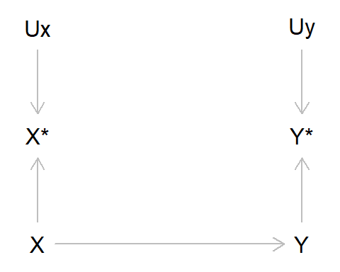
Let’s unpack this DAG a bit, as there are quite a few new elements here:
- Here, we are saying that the true value of X causes the true value of Y
- However, as X and Y are imperfectly measured, we only have the observed variables X* and Y*
- These observed values are caused by the true values (as we would hope!), but are also caused by measurement error UX and UY
In reality, this means that in our model with the observed data, we are no longer measuring the association between X and Y, but rather we are measuring the association between X* and Y* . As X* may not be the same as X - and Y* not the same as Y - there is the possibility that error may have crept into our measurements. Such measurement error will frequently result in bias, although the magnitude and direction of this bias will depend on various factors.
Types of measurement error: Differential and dependent
There are two main types of measurement error: whether measurement error is differential or non-differential, and whether measurement error is dependent or independent.
Whether error is differential or not depends on whether the error in one variable is caused by the values of other variables. Say our exposure is alcohol intake and our outcome is liver disease, and alcohol intake was measured retrospectively in a case-control design of individuals with vs without liver disease. In this example, those with liver disease may recall drinking more alcohol when younger, as a consequence of contracting liver disease; in this case, measurement error in alcohol intake will be differential, as the error will depend on the value of the outcome. If alcohol intake and liver disease were measured independently in a prospective cohort study, say, with alcohol intake measured prior to liver disease diagnosis, then liver disease cannot cause measurement error in the exposure, and any measurement error would be non-differential.
Whether error is dependent or independent is due to whether the errors - UX and UY - are correlated or not. In the DAG above UX and UY are independent, as the errors in X* are unrelated to the errors in Y*. But if the errors have a common cause, as we will see below, then they will be dependent. An example may be a survey asking about illegal drug use and mental health. If these were asked at the same time, then perhaps respondents would under-report both drug use and mental health symptoms, meaning that errors in these variables would be correlated, and hence dependent. If these data came from different sources - say, drug use from a survey and mental health from health-care records - then measurement error would likely be independent, as error in one variable would be independent of error in another variable.
These terms will be explained and described in more detail below, but for now they are just being introduced to be aware of the terminology. Together, these combinations of differential and dependent measurement error, result in four combinations of measurement error: non-differential and independent, differential and independent, non-differential and dependent, and differential and dependent.
We’ll start with non-differential and independent measurement error, as it’s the simplest place to start.
Non-differential measurement error
As mentioned above, measurement error is differential when the error in one variable depends on the values of another variable, and non-differential if the error in one variable does not depend on the values of another.
If measurement error is non-differential and independent, then the DAG above represents the structure of measurement error; in other words, both X and Y are imperfectly measured, but error in one variable is unrelated to the other variable. Even in this scenario, and where the only thing affecting measurement error is random noise, our results are nonetheless going to be biased. The following R code demonstrates this using two binary variables, in situations where there is no measurement error, measurement error in X only, measurement error in Y only, and measurement error in both X and Y (comparable Stata code can be found at the end of the blog).
## Set the seed so data is reproducible
set.seed(543210)

## Simulate exposure 'X'
x <- rbinom(n = 10000, size = 1, prob = 0.5)

## Simulate outcome 'Y' (say that risk of outcome
## is double if exposure == 1)
y <- ifelse(x == 0, rbinom(n = sum(x == 0),
                           size = 1, prob = 0.25),
            rbinom(n = sum(x == 1), size = 1, prob = 0.5))

## Table of true X and Y, and calculate risk ratio
table(x, y)
## y
## x 0 1
## 0 3838 1222
## 1 2440 2500(sum(x == 1 & y == 1) / sum(x == 1)) /
(sum(x == 0 & y == 1) / sum(x == 0))## [1] 2.095523## Add some measurement error to X (10% of
## cases are incorrectly categorised)
x_error <- ifelse(x == 0, rbinom(n = sum(x == 0),
size = 1, prob = 0.1),
rbinom(n = sum(x == 1),
size = 1, prob = 0.9))
## Table of X with measurement error and true Y,
## and calculate risk ratio
table(x_error, y)## y
## x_error 0 1
## 0 3670 1362
## 1 2608 2360(sum(x_error == 1 & y == 1) / sum(x_error == 1)) /
(sum(x_error == 0 & y == 1) / sum(x_error == 0))## [1] 1.755068## Add some measurement error to Y (again,
## 10% of cases incorrectly categorised)
y_error <- ifelse(y == 0, rbinom(n = sum(y == 0),
size = 1, prob = 0.1),
rbinom(n = sum(y == 1),
size = 1, prob = 0.9))
## Table of true X and Y with measurement error,
## and calculate risk ratio
table(x, y_error)## y_error
## x 0 1
## 0 3567 1493
## 1 2439 2501(sum(x == 1 & y_error == 1) / sum(x == 1)) /
(sum(x == 0 & y_error == 1) / sum(x == 0))## [1] 1.715843## Table of X and Y both with measurement error,
## and calculate risk ratio
table(x_error, y_error)## y_error
## x_error 0 1
## 0 3428 1604
## 1 2578 2390(sum(x_error == 1 & y_error == 1) / sum(x_error == 1)) /
(sum(x_error == 0 & y_error == 1) / sum(x_error == 0))## [1] 1.50922We can also explore the impact of non-differential measurement error for continuous variables:
## Set the seed so data is reproducible
set.seed(543210)

## Simulate exposure 'X'
x <- rnorm(n = 10000, mean = 0, sd = 1)

## Simulate outcome 'Y' (say that correlation is about 0.5)
y <- (0.57 * x) + rnorm(n = 10000, mean = 0, sd = 1)

## Correlation of true X and Y
cor(x, y)
## [1] 0.5031961## Add some measurement error to X (mean of 0 and
## SD of 0.5)
x_error <- x + rnorm(n = 10000, mean = 0, sd = 0.5)
## Correlation of X with measurement error and true Y
cor(x_error, y)## [1] 0.4534758## Add some measurement error to Y (again,
## mean of 0 and SD of 0.5)
y_error <- y + rnorm(n = 10000, mean = 0, sd = 0.5)
## Correlation of true X and Y with measurement error
cor(x, y_error)## [1] 0.467734## Correlation of X and Y both with measurement error
cor(x_error, y_error)## [1] 0.4234048For all these examples, non-differential measurement error results in a bias towards the null (an exception is the case where the true X - Y effect is null, in which case non-differential measurement error does not result in bias as the association is already null). While this is a widely-reported rule-of-thumb, it is important to note that there are several exceptions to this rule, such as if there are more than two values of a categorical variable, in the presence of dependent measurement error, and if there is confounder misclassification, in addition to other circumstances.5
Okay, so that’s non-differential measurement error, which often - but by no means always! - results in bias towards the null. Non-differential error is the simplest form of measurement error - Let’s now turn to differential measurement error, where things get a bit more complicated.
Differential measurement error
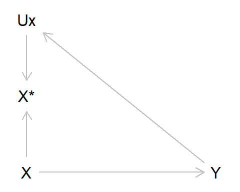
To re-cap, differential measurement error occurs when the error in one variable depends on the value of another. Earlier we gave the example of recall bias in a case-control study of alcohol intake as our exposure and liver disease as our outcome; those with liver disease may recall drinking more alcohol earlier in life, due to their subsequent diagnosis. Using the standard measurement error DAG above, we can adapt this by adding an arrow from Y to UX, indicating that the value of liver disease diagnosis alters measurement error in alcohol intake. As can be seen from the DAG, there is an open path from X* -> UX -> Y, indicating that this association will be biased. In this example we’ll also assume no measurement error in Y (hence why Y* and UY do not appear in the DAG below).
As per usual, let’s simulate some data to illustrate this:
## Set the seed so data is reproducible
set.seed(54321)

## Simulate true alcohol intake exposure (as binary
## 1 = high vs 0 = low, for simplicity)
alc <- rbinom(n = 10000, size = 1, prob = 0.25)

## Simulate outcome liver disease (say that risk is
## 3 times higher if high alcohol intake)
liver <- ifelse(alc == 0, rbinom(n = sum(alc == 0),
                                 size = 1, prob = 0.05),
                rbinom(n = sum(alc == 1),
                       size = 1, prob = 0.15))

## Table of true alcohol intake and liver disease,
## and calculate risk ratio
table(alc, liver)
## liver
## alc 0 1
## 0 7149 372
## 1 2098 381(sum(alc == 1 & liver == 1) / sum(alc == 1)) /
(sum(alc == 0 & liver == 1) / sum(alc == 0))## [1] 3.107285## Next, simulate observed alcohol intake, where those
## with liver disease over-report their prior consumption
## (say, those with liver disease are 10% more likely to claim
## to have had high alcohol consumption, if in fact it was low)
alc_error <- ifelse(alc == 0 & liver == 1,
rbinom(n = sum(alc == 0 & liver == 1),
size = 1, prob = 0.1), alc)
## Table of alcohol intake with error and true liver disease,
## and calculate risk ratio
table(alc_error, liver)## liver
## alc_error 0 1
## 0 7149 330
## 1 2098 423(sum(alc_error == 1 & liver == 1) / sum(alc_error == 1)) /
(sum(alc_error == 0 & liver == 1) / sum(alc_error == 0))## [1] 3.802744In this example, differential measurement error has resulted in a change in the risk ratio from approximately 3 to nearly 4, a large shift away from both the true value and - in contrast to non-differential error - away from the null. The direction of measurement bias due to differential error is therefore more difficult to predict than for non-differential error, as it could be either towards or away from the null, depending on the specific relations between variables (in the example above, if the outcome caused a reduction in the probability of answering ‘high alcohol intake’, then the bias would be a reduction in the effect estimate, towards the null).
The same dynamics also occur if the exposure causes error in the outcome. Let’s return to the example of Samuel George Morgan and the measurement of skull volume from different populations. Here, our exposure is the population the skull came from, our outcome is the skull volume, and there is an arrow from the exposure to the measurement error of the outcome as the skull volumes of White Europeans are biased upwards. We are assuming there is no true causal effect of population on skull size in this example, hence the lack of arrow from ‘population’ to ‘skullSize’. As above, we are again assuming that there is no measurement error in which population the skulls came from.

Let’s simulate this up:
## Set the seed so data is reproducible
set.seed(54321)

## Simulate true population exposure (as binary
## 1 = White European vs 0 = Rest of world)
pop <- rbinom(n = 100, size = 1, prob = 0.5)

## Simulate outcome skull volume (not caused
## by population; in cm^3)
skull <- rnorm(n = 100, mean = 1400, sd = 100)

## Difference in brain volume between populations
## using true data
mod_skull <- lm(skull~ pop)
cbind(pop = coef(summary(mod_skull))[, 1],
      confint(mod_skull))["pop", ]
## pop 2.5 % 97.5 %
## 13.08476 -26.96563 53.13514## Add some experimenter bias in, where skull volume
## of White European's increased by 25 cm^3, while
## is decreased by same amount in the rest of the world
skull_error <- ifelse(pop == 1, skull[pop == 1] +
rnorm(n = sum(pop == 1),
mean = 25, sd = 50),
skull[pop == 0] - rnorm(n = sum(pop == 0),
mean = 25, sd = 50))
## Difference in brain volume between populations
## using biased data
mod_skull_error <- lm(skull_error ~ pop)
cbind(pop = coef(summary(mod_skull_error))[, 1],
confint(mod_skull_error))["pop", ]## pop 2.5 % 97.5 %
## 56.81449 15.54401 98.08497Now, even though there were no differences in skull size between the populations in the true data, with this differential bias we can see that skulls of White Europeans are larger than those from other parts of the world.
So far, we have treated differential and non-differential measurement error in isolation, but they can also work together. Say that someone played a joke on Morgan and relabelled some of his skulls, so that 20% of the White European skulls were labelled as ‘rest of the world’, and vice versa for 20% of skulls from the rest of the world being labelled as ‘White European’. The DAG would now look like this:

And we simulate this like so (note that this is carried on from the same code chunk above):
## Combine this experimenter bias with some non-differential
## measurement error in the exposure
pop_error <- ifelse(pop == 1, rbinom(n = sum(pop == 1),
                                     size = 1, prob = 0.8),
                    rbinom(n = sum(pop == 0),
                           size = 1, prob = 0.2))

## Difference in brain volume between populations
## using biased data (plus non-diff error in exposure)
mod_skull_error2 <- lm(skull_error ~ pop_error)
cbind(pop = coef(summary(mod_skull_error2))[, 1],
      confint(mod_skull_error2))["pop_error", ]
## pop 2.5 % 97.5 %
## 25.24484 -17.69083 68.18051Here the differential and non-differential measurement error work in opposite directions: The differential error results in an illusory increase in skull size difference between the populations, while the non-differential error in the population assignment attenuates this bias back towards the null.
Hopefully this example has illustrated how difficult it can be to determine the magnitude and direction of measurement bias, even in an incredibly simplistic scenario such as this, which only considers a single exposure and outcome, so ignores any issues of selection or confounding bias, or other sources of measurement bias such as dependent measurement errors. It is this latter source of measurement bias to which we now turn.
Dependent Measurement Error
Up to now, we have been focusing on differential and non-differential error, while assuming that the errors themselves are independent of one another. If the data come from different sources - say, the exposure from a questionnaire and the outcome from medical records - then the assumption of independent errors may be valid. This is the original DAG in this post, where UX and UY do not share a common cause.
If data originate from the same source, however, then it is possible that the errors will be dependent, and can be represented like so, with the common source of error UXY causing both UX and UY.

As an example, when answering a questionnaire some individuals might under- or over-report both whether they experienced stressful life events and symptoms of depression, in which case measurement error would be dependent between these variables. Here’s a simple simulation to show how this can bias results, giving examples where some of those who experienced stressful life events and had depression under-reported these, and where some of those who had not experienced stressful life events or had depression over-reported these:
## Set the seed so data is reproducible
set.seed(654321)

## Simulate true stressful life events exposure
## (as binary)
events <- rbinom(n = 10000, size = 1, prob = 0.2)

## Simulate outcome depression (caused by life
## events; again, code as binary)
dep_p <- plogis(log(0.1) + (log(2) * events))
dep <- rbinom(n = 10000, size = 1, prob = dep_p)

table(events, dep)
## dep
## events 0 1
## 0 7302 724
## 1 1637 337## Effect of life events on depression using
## true data
mod_dep <- glm(dep ~ events, family = "binomial")
exp(cbind(events = coef(summary(mod_dep))[, 1],
confint(mod_dep))["events", ])## Waiting for profiling to be done...## events 2.5 % 97.5 %
## 2.076273 1.803610 2.386221## Add some dependent error in, by saying that 10% of
## people are less likely to answer that life events
## were stressful and report fewer depressive symptoms,
## if both of these did in fact occur
error <- ifelse(events == 1 & dep == 1,
rbinom(n = sum(events == 1 & dep == 1),
size = 1, prob = 0.1), 0)
events_error <- ifelse(error == 1, 0, events)
dep_error <- ifelse(error == 1, 0, dep)
table(events_error, dep_error)## dep_error
## events_error 0 1
## 0 7364 724
## 1 1637 275## Effect of life events on depression using
## data with dependent error
mod_dep_error <- glm(dep_error ~ events_error,
family = "binomial")
exp(cbind(events = coef(summary(mod_dep_error))[, 1],
confint(mod_dep_error))["events_error", ])## Waiting for profiling to be done...## events 2.5 % 97.5 %
## 1.708674 1.470553 1.980514## Could also get reverse, where some people who were
## not exposed to a stressful event or depressed rated
## these as present
error2 <- ifelse(events == 0 & dep == 0,
rbinom(n = sum(events == 0 & dep == 0),
size = 1, prob = 0.01), 0)
events_error2 <- ifelse(error2 == 1, 1, events)
dep_error2 <- ifelse(error2 == 1, 1, dep)
table(events_error2, dep_error2)## dep_error2
## events_error2 0 1
## 0 7218 724
## 1 1637 421## Effect of life events on depression using
## data with dependent error
mod_dep_error2 <- glm(dep_error2 ~ events_error2,
family = "binomial")
exp(cbind(events = coef(summary(mod_dep_error2))[, 1],
confint(mod_dep_error2))["events_error2", ])## Waiting for profiling to be done...## events 2.5 % 97.5 %
## 2.563963 2.246733 2.923168As can be seen from the results above, the direction of dependent error can bias results either towards or away from the null, depending on the structure of these dependent errors. Things become a great deal more complicated when considering both differential and dependent error jointly, and it can be very difficult to predict the direction and magnitude of the bias due to measurement error in these situations.
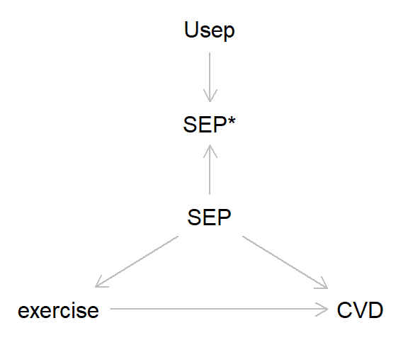
Measurement error in confounding variables
So far in this blog we’ve focused on the simplest cases with just a single exposure and outcome. However, in most analyses we’d probably want to control for various confounding factors, and here measurement error can also lead to bias. Take the DAG below, where the association between exercise and cardiovascular disease (CVD) is confounded by socioeconomic position (SEP). Let’s say - miraculously! - that exercise and CVD are measured without error, while SEP has some non-differential measurement error. Here’s the DAG:
And here’s some code to simulate this:
## Set the seed so data is reproducible
set.seed(7654321)

## Simulate true SEP
high_sep <- rbinom(n = 10000, size = 1, prob = 0.5)

## Simulate exposure exercise (caused by SEP;
## hours per week)
exercise <- 5 + (2 * high_sep) +
  rnorm(n = 10000, mean = 0, sd = 1)
summary(exercise)
## Min. 1st Qu. Median Mean 3rd Qu. Max.
## 1.303 4.975 6.004 6.004 7.052 10.494## Simulate outcome CVD (caused by SEP and exercise;
## higher SEP and exercise = lower rate of CVD)
cvd_p <- plogis(log(0.25) + (log(0.5) * high_sep) +
(log(0.8) * exercise))
cvd <- rbinom(n = 10000, size = 1, prob = cvd_p)
table(cvd)## cvd
## 0 1
## 9448 552## Effect of exercise on CVD, not adjusting for SEP, using
## true data
mod_noSEP <- glm(cvd ~ exercise, family = "binomial")
exp(cbind(exercise = coef(summary(mod_noSEP))[, 1],
confint(mod_noSEP))["exercise", ])## Waiting for profiling to be done...## exercise 2.5 % 97.5 %
## 0.7018851 0.6584133 0.7477897## Effect of exercise on CVD, adjusting for SEP, using
## true data
mod_true <- glm(cvd ~ exercise + high_sep, family = "binomial")
exp(cbind(exercise = coef(summary(mod_true))[, 1],
confint(mod_true))["exercise", ])## Waiting for profiling to be done...## exercise 2.5 % 97.5 %
## 0.8157251 0.7476991 0.8898338## Add some non-differential error to the confounder SEP
sep_error <- ifelse(high_sep == 1,
rbinom(n = sum(high_sep == 1),
size = 1, prob = 0.9),
rbinom(n = sum(high_sep == 0),
size = 1, prob = 0.1))
table(high_sep, sep_error)## sep_error
## high_sep 0 1
## 0 4533 435
## 1 511 4521## Effect of exercise on CVD, adjusting for SEP, using
## SEP data with error
mod_error <- glm(cvd ~ exercise + sep_error, family = "binomial")
exp(cbind(exercise = coef(summary(mod_error))[, 1],
confint(mod_error))["exercise", ])## Waiting for profiling to be done...## exercise 2.5 % 97.5 %
## 0.7590974 0.7034203 0.8188950In this example, because SEP causes higher rates of exercise and lower rates of CVD, including SEP-with-error in the model results in bias away from the null, and closer to the effect estimate between exercise and CVD where SEP is not adjusted for. This is because measurement error in SEP means that we are not adequately adjusting for the effect of this confounder.6 Again, depending on the structure of confounding and the causes of bias in the confounder, the direction and magnitude of the resulting bias could be hard to predict.
What can be done about measurement bias?
Measurement error, and its resulting bias, can stem from numerous sources, ranging from conceptual errors (not measuring the intended construct very well), recording errors (e.g., recall, self-report of interviewer bias), or just plain old data management errors. As with pretty much all stats advice, the key is to carefully think through all of these sources of error prior to collecting data. For instance:
- Is my question/variable measuring what I want it to? If your intended outcome is ‘intelligence’, then asking a validated battery of IQ measures is probably preferable to simply asking about educational attainment (even if they are correlated)
- Is there a less error-prone measure I can use? Self-report measures of some variables are likely to be more error-prone than more ‘objective’ assessments from clinic assessments, especially for measures like height, weight, BMI, etc.
- Is there a risk of differential error? If the way you are asking about your exposure and outcome (and other covariates) may bias responses to some of the other variables, then measurement error may result in bias. This may be a particular issue for retrospective studies relying on recall - as with the example of alcohol intake and liver disease - but can impact other research designs too.
- Is there a risk of dependent error? If measurement errors may be correlated when taken from the same source (e.g., self-reported questionnaires), then consider using different sources of information (e.g., self-reported questionnaire data for the exposure, and biomarker or health record data for the outcome)
Of course, even with the most careful planning measurement error may still be an issue. In these cases, there are various bias analyses that have been developed for quantifying and assessing the potential impact of measurement bias. Many of these rely on using a subset of validated data to explore measurement bias (e.g., comparing self-reported weights to a subset of clinic-measured weights, or self-reported prescription drug use to prescriptions from health records). See the further reading section for more info on these kinds of quantitative bias analyses for measurement error.
Summary
In this post we have introduced the concept of measurement bias (or information bias), which can occur when measured variables differ from their true value. Two sources of measurement bias are whether measurement error is differential or non-differential (i.e., whether measurement error is caused by the values of other variables), and whether measurement error is dependent or independent (i.e., whether measurement error in one variable is correlated with error in another variable). As we have seen, the bias resulting from these sources of measurement error can be quite substantial, and the direction of said bias often difficult to predict. And even in the simplest of scenarios - non-differential and independent errors - the heuristic that measurement error will always attenuate the true effect towards the null may not always be correct.
In addition to confounding and selection/collider bias, measurement bias is the third source of bias that may result in spurious associations and incorrect causal inferences. Although generally overlooked relative to confounding and selection, given its ubiquity in all types of research measurement error is a crucial factor which ought to be considered in all studies.
In the next post, I’ll bring together all the threads of the previous posts, and try to make one final case for taking a causal perspective when conducting research.
Further Reading
There are a number of great introductions to measurement error and bias, here are a few I’ve found particularly useful:
- Chapter 13 of Modern Epidemiology on ‘Measurement and measurement error’ by Lash, VanderWeele and Rothman is a great introduction to all things measurement bias-related.
- This recent paper by Innes and colleagues is another nice introduction to measurement error, including some approaches for overcoming measurement bias.
- Chapter 9 of Miguel Hernán and Jamie Robins’ book Causal Inference: What If is another fab intro to measurement bias.
- There have also been some recent papers busting myths about measurement error - such as ‘non-differential error also biases towards the null’ - including here and here.
- The classic paper on measurement error in covariates is this 1980 paper by Greenland.
Stata code
*** Non-differential measurement error (binary)

* Clear data, set observations and set seed
clear
set obs 10000
set seed 543210

* Simulate exposure 'X'
gen x = rbinomial(1, 0.5)

* Simulate outcome 'Y' (say that risk of outcome
* is double if exposure == 1)
gen y = rbinomial(1, 0.25) if x == 0
replace y = rbinomial(1, 0.5) if x == 1

* Table of true X and Y, and calculate risk ratio
tab x y
glm y x, family(binomial) link(log) eform noheader

* Add some measurement error to X (10% of
* cases are incorrectly categorised)
gen x_error = rbinomial(1, 0.1) if x == 0
replace x_error = rbinomial(1, 0.9) if x == 1

* Table of X with measurement error and true Y,
* and calculate risk ratio
tab x_error y
glm y x_error, family(binomial) link(log) eform noheader

* Add some measurement error to Y (again,
* 10% of cases incorrectly categorised)
gen y_error = rbinomial(1, 0.1) if y == 0
replace y_error = rbinomial(1, 0.9) if y == 1

* Table of true X and Y with measurement error,
* and calculate risk ratio
tab x y_error
glm y_error x, family(binomial) link(log) eform noheader

* Table of X and Y both with measurement error,
* and calculate risk ratio
tab x_error y_error
glm y_error x_error, family(binomial) link(log) eform noheader


*** Non-differential measurement error (continuous)

* Clear data, set observations and set seed
clear
set obs 10000
set seed 543210

* Simulate exposure 'X'
gen x = rnormal(0, 1)

* Simulate outcome 'Y' (say that correlation is about 0.5)
gen y = (0.57 * x) + rnormal(0, 1)

* Correlation of true X and Y
cor x y

* Add some measurement error to X (mean of 0 and
* SD of 0.5)
gen x_error = x + rnormal(0, 0.5)

* Correlation of X with measurement error and true Y
cor x_error y

* Add some measurement error to Y (again,
* mean of 0 and SD of 0.5)
gen y_error = y + rnormal(0, 0.5)

* Correlation of true X and Y with measurement error
cor x y_error

* Correlation of X and Y both with measurement error
cor x_error y_error


*** Differential measurement error (alcohol and liver disease;
*** differential based on outcome)

* Clear data, set observations and set seed
clear
set obs 10000
set seed 54321

* Simulate true alcohol intake exposure (as binary
* 1 = high vs 0 = low, for simplicity)
gen alc = rbinomial(1, 0.25)

* Simulate outcome liver disease (say that risk is
* 3 times higher if high alcohol intake)
gen liver = rbinomial(1, 0.05) if alc == 0
replace liver = rbinomial(1, 0.15) if alc == 1

* Table of true alcohol intake and liver disease,
* and calculate risk ratio
table(alc, liver)
glm liver alc, family(binomial) link(log) eform noheader


* Next, simulate observed alcohol intake, where those
* with liver disease over-report their prior consumption
* (say, those with liver disease are 10% more likely to claim
* to have had high alcohol consumption, if in fact it was low)
gen alc_error = alc if alc == 1 | liver == 0
replace alc_error = rbinomial(1, 0.1) if alc == 0 & liver == 1

* Table of alcohol intake with error and true liver disease,
* and calculate risk ratio
tab alc_error liver
glm liver alc_error, family(binomial) link(log) eform noheader


*** Differential measurement error (race and skull size;
*** differential based on exposure)

* Clear data, set observations and set seed
clear
set obs 100
set seed 54321

* Simulate true population exposure (as binary
* 1 = White European vs 0 = Rest of world)
gen pop = rbinomial(1, 0.5)

* Simulate outcome skull volume (not caused
* by population; in cm^3)
gen skull = rnormal(1400, 100)

* Difference in brain volume between populations
* using true data
regress skull pop

* Add some experimenter bias in, where skull volume
* of White European's increased by 25 cm^3, while
* is decreased by same amount in the rest of the world
gen skull_error = skull + rnormal(25, 50) if pop == 1
replace skull_error = skull - rnormal(25, 50) if pop == 0

* Difference in brain volume between populations
* using biased data
regress skull_error pop

* Combine this experimenter bias with some non-differential
* measurement error in the exposure
gen pop_error = rbinomial(1, 0.8) if pop == 1
replace pop_error = rbinomial(1, 0.2) if pop == 0

* Difference in brain volume between populations
* using biased data (plus non-diff error in exposure)
regress skull_error pop_error


*** Dependent measurement error (life events and depression)

* Clear data, set observations and set seed
clear
set obs 10000
set seed 654321

* Simulate true stressful life events exposure
* (as binary)
gen events = rbinomial(1, 0.2)

* Simulate outcome depression (caused by life
* events; again, code as binary)
gen dep_p = invlogit(log(0.1) + (log(2) * events))
gen dep = rbinomial(1, dep_p)

tab events dep

* Effect of life events on depression using
* true data
logistic dep events

* Add some dependent error in, by saying that 10% of
* people are less likely to answer that life events
* were stressful and report fewer depressive symptoms,
* if both of these did in fact occur
gen error = 0
replace error = rbinomial(1, 0.1) if events == 1 & dep == 1

gen events_error = events
replace events_error = 0 if error == 1
gen dep_error = dep
replace dep_error = 0 if error == 1
tab events_error dep_error

* Effect of life events on depression using
* data with dependent error
logistic dep_error events_error

* Could also get reverse, where some people who were
* not exposed to a stressful event or depressed rated
* these as present
gen error2 = 0
replace error2 = rbinomial(1, 0.01) if events == 0 & dep == 0

gen events_error2 = events
replace events_error2 = 1 if error2 == 1
gen dep_error2 = dep
replace dep_error2 = 1 if error2 == 1
tab events_error2 dep_error2

* Effect of life events on depression using
* data with dependent error
logistic dep_error2 events_error2


*** Measurement error in confounders

* Clear data, set observations and set seed
clear
set obs 10000
set seed 7654321

* Simulate true SEP
gen high_sep = rbinomial(1, 0.5)

* Simulate exposure exercise (caused by SEP;
* hours per week)
gen exercise = 5 + (2 * high_sep) + rnormal(0, 1)
sum exercise

* Simulate outcome CVD (caused by SEP and exercise)
gen cvd_p = invlogit(log(0.01) + (log(2) * high_sep) + ///
                      (log(1.25) * exercise))
gen cvd = rbinomial(1, cvd_p)
tab cvd

* Effect of exercise on CVD, not adjusting for SEP, using
* true data
logistic cvd exercise

* Effect of exercise on CVD, adjusting for SEP, using
* true data
logistic cvd exercise high_sep

* Add some non-differential error to the confounder SEP
gen sep_error = rbinomial(1, 0.9) if high_sep == 1
replace sep_error = rbinomial(1, 0.1) if high_sep == 0
tab high_sep sep_error

* Effect of exercise on CVD, adjusting for SEP, using
* SEP data with error
logistic cvd exercise sep_error
In addition to all the other questionable research practices which can be used to support one’s own pet theory - p-hacking, selective reporting, file-drawer effect/publication bias, fraudulent data, etc. etc.↩︎
In another twist to this tale, critiques of Gould’s re-analysis have subsequently been published, suggesting that Gould’s own biases may have gone too far the other way and obscured any group-level differences - these (re-)re-analyses have been debated and critiqued, however, so it’s not really clear what to make of everything. For a detailed discussion, see here and references therein to go down this rabbit-hole.↩︎
That said, many of the differences between Gould and Morgan are in fact not just due to measurement error, but rather analysis choices - which skulls to include or exclude, etc. - which I won’t go into here.↩︎
Not to mention ‘white coat hypertension’, where the stress of being in a clinic environment can raise blood pressure.↩︎
For a recent paper on bias from non-differential measurement error, see here. Also, if X is categorical and Y is continuous, then non-differential error in Y will not result in bias (but will result in greater uncertainty; see this paper for more info) - I’ll leave this as an exercise to the reader to test out.↩︎
You could think of this example as either an example of measurement bias, or of unmeasured confounding - Both perspectives are equally valid.↩︎