Dagatha Christie and the Secret of the Colliding Variables (5)

Defining ‘collider bias’

We’ll get back to this curious case in a minute. But first we need to understand what collider bias is. Collider bias occurs when one conditions on a common consequence of (i.e., a variable caused by) the exposure and outcome (or factors related to the exposure and outcome). A ‘collider’ is a variable caused by two or more variables - as these variables ‘collide’ at said third variable; colliders are easy to spot in DAGs, as they have two or more arrows pointing towards them.

This all sounds rather abstract, so let’s draw a DAG to make this conceptually clearer.

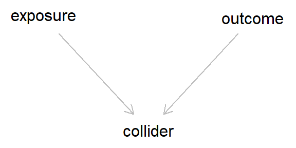
This is the caononical DAG for collider bias (although more complex scenarios can also result in collider bias, as we’ll see below). This still looks rather innocuous, but a lot of damage can occur due to these colliders. Essentially, even though there is no arrow between the exposure and the outcome - meaning that the exposure does not cause the outcome - as both the exposure and outcome cause the collider, if we condition on (i.e., adjust for) said collider, we would induce a spurious association between the exposure and outcome.

In this scenario, we would get a correlation between two variables without any causation!

Demonstrating collider bias

This is still pretty abstract and unintuitive. But the lesson to learn for now is that conditioning on a collider can lead to bias, and in turn result in erroneous inferences. Like confounding, collider bias can also result in bias, but it is much less familiar to most researchers than the more recognisable bias resulting from confounding.

Let’s explore this example in a bit more detail to try and add some intuition to how this can result in bias. We’ll use the example of an actor’s skill and their attractiveness in getting famous as an illustrative example.

First, we’ll simply demonstrate that conditioning on a collider can result in bias. Here, we’re treating ‘acting skill’ and ‘attractiveness’ as normally-distributed variables which are independent from one another (of course, you can’t really measure these traits quantitatively along just one dimension, but humour me for now). Then, we say that actors who are either highly skilled or very attractive are more likely to become famous (with 5 times greater of being famous for each unit increase in skill and attractiveness). Here’s some R code to simulate this simple scenario (Stata code can be found at end of the blog).

## Set the seed so data is reproducible
set.seed(54321)

## Simulate 'acting skill' (caused by nothing)
skill <- rnorm(n = 10000, mean = 0, sd = 1)

## Simulate attractiveness (again, caused by nothing)
attract <- rnorm(n = 10000, mean = 0, sd = 1)

## And now simulate 'becoming famous' (as a binary
## variable; caused by both skill and attractiveness)
famous_p <- plogis(log(0.05) + (log(5) * skill)
                   + (log(5) * attract))
famous <- rbinom(n = 10000, size = 1, prob = famous_p)
table(famous)

## famous
##    0    1 
## 8566 1434

Now that we’ve simulated the data, let’s check that acting skill and attractiveness are completely independent of one another.

mod <- lm(attract ~ skill)

# Summary of association
cbind(skill = coef(summary(mod))[, 1], 
          confint(mod))["skill", ]

##        skill        2.5 %       97.5 % 
## -0.006541693 -0.026064974  0.012981588

Great, there’s no association! (just as we simulated)

Now, let’s include ‘famous’ as a covariate in the model

mod_collide <- lm(attract ~ skill + famous)

# Summary of association
cbind(skill = coef(summary(mod_collide))[, 1], 
          confint(mod_collide))["skill", ]

##      skill      2.5 %     97.5 % 
## -0.1460978 -0.1652115 -0.1269840

Okay, so now there’s a strong negative association between acting skill and attractiveness. This is odd, as we know in ‘truth’ that there is no causal relationship between acting skill and attractiveness…

This is due to collider bias, because both ‘acting skill’ and ‘attractiveness’ cause one to be famous; that is, both of these variables ‘collide’ with ‘famous’. Updating the DAG above should make this a bit clearer.

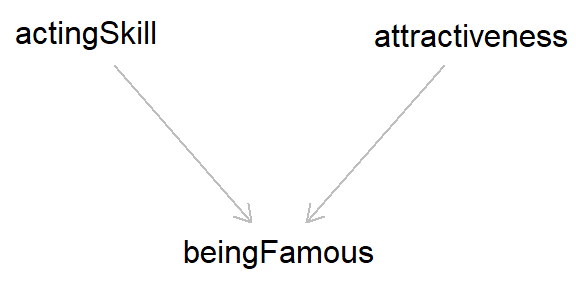
As both ‘acting skill’ and ‘attractiveness’ cause fame, if we adjust for this collider (‘famous’) we induce a spurious association between these variables (in DAGs, adjusting for/conditioning on a variable is usually designated by a box around said variable). However, if we do not adjust for fame, then we return the true - and in this case, null - association between ‘skill’ and ‘attractiveness’. So collider bias can give the illusion of association, even without causation. Pretty worrying, right??³

In the example above I’ve shown how collider bias can occur when explicitly adjusting for a collider variable in a regression model. But things can get even more worrying when we realise that collider bias can occur implicitly in an analysis based on study design, or non-random participant recruitment and/or drop-out (missing data, in other words). Let’s say that our sample consists solely of famous actors. In this example, we are implicitly conditioning on being famous, so we again observe a negative association between acting skill and attractiveness.

mod_collide <- lm(attract ~ skill, subset = famous == 1)

# Summary of association
cbind(skill = coef(summary(mod_collide))[, 1], 
          confint(mod_collide))["skill", ]

##      skill      2.5 %     97.5 % 
## -0.3085037 -0.3602856 -0.2567218

We can display this in a plot, to make this even clearer to see. In this plot, the ‘famous’ people are coded in red, with the non-famous people in black. The blue line is the association between acting skill and attractiveness in the full sample (i.e., the true effect, which is clearly null), while the red line is the association between acting skill and attractiveness among famous individuals (i.e., the biased association, which is clearly negative).

plot(attract ~ skill, pch = 1, lwd = 2, col = factor(famous),
     xlab = "Acting skill", ylab = "Attractiveness")
abline(mod, col = "blue", lwd = 3)
abline(mod_collide, col = "red", lwd = 3)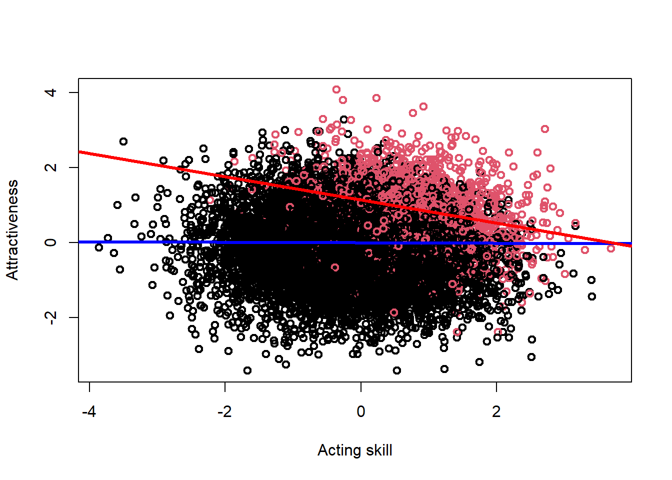

If we were not aware of collider bias, from a study such as this we might therefore conclude that there is a - potentially causal - negative association between acting skill and attractiveness. However, here we know that this spurious association is just an artifact of our biased sampling procedure. Similar concerns can affect longitudinal studies, where non-random enrolment and/or drop-out over time can result in collider bias and potentially erroneous inferences.

Explaining collider bias

Okay, so we’ve demonstrated that collider bias does occur and it’s something the researchers should both know and worry about. But why does it occur? It almost seems a bit like Einstein’s ‘spooky action at a distance’, where variables appear to affect one another despite no causal connections between them. This bias occurs because, once we condition on a collider, knowing the value of one variable tells us information about another. This is still rather obscure, so let’s use a simple example as a nice intuition pump.

Imagine there is a bell and two coins. Both coins are flipped, and if either coin ends up ‘heads’, the bell rings. These are unbiased coins, so they are completely independent from one another. This situation corresponds to the canonical ‘collider bias’ DAG introduced above.

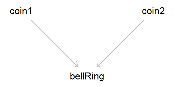
Now, say that we look at the association between the result of both coin tosses, conditioning on when the bell has rung. Once the bell has rung, if one of the coins is ‘tails’, that means that the other must be ‘heads’ (else the bell would not have rung). Even though the coin tosses are independent, when conditioning on the bell ringing the two coins become dependent, as the value of one coin provides information about the other (in this case, we induce a negative association between the coin tosses, as if one coin is ‘tails’ then the other must be ‘heads’).

The same logic explains all other cases of collider bias as well. Taking the ‘acting skill’, ‘attractiveness’ and ‘fame’ example from above, if we condition on ‘fame’ we induce a spurious negative association between acting skill and attractiveness. This is because, of those who are ‘famous’, if we know that person is skilled, then that information also tells us that they are less likely to be attractive. The same reasoning applies to attractive famous people: if we know they’re attractive, then that gives us information about their acting skill (i.e., that it’s going to be lower). The same reasoning applies in both the ‘famous’ and ‘non-famous’ strata, as there is a negative association present in both.

## Conditioning on being famous
mod_collide <- lm(attract ~ skill, subset = famous == 1)

# Summary of association
cbind(skill = coef(summary(mod_collide))[, 1], 
          confint(mod_collide))["skill", ]

##      skill      2.5 %     97.5 % 
## -0.3085037 -0.3602856 -0.2567218

## Conditioning on not being famous
mod_collide2 <- lm(attract ~ skill, subset = famous == 0)

# Summary of association
cbind(skill = coef(summary(mod_collide2))[, 1], 
          confint(mod_collide2))["skill", ]

##      skill      2.5 %     97.5 % 
## -0.1246272 -0.1451675 -0.1040868

Don’t worry if you’re struggling with this explanation, collider bias is quite a counter-intuitive concept, and I still get myself confused when thinking about how collider bias works from time to time. I find that the coin and bell-ringing example is the simplest example to understand how conditioning on a collider can lead to a dependency between two independent variables, so relating examples back to that may help.

Smoking and COVID-19 as case-study of collider bias

Okay, hopefully that’s enough background to collider bias, and you all have an appreciation (and hopefully a vague understanding) for how collider bias can result in spurious associations. Now we’ll return to the example that started this blog: smoking, COVID-19 and hospitalisation.

Early reports during the COVID-19 pandemic suggested that smoking may be protective against COVID-19. That is, among hospitalised patients rates of COVID-19 were lower among smokers than non-smokers. Given what we’ve discussed above, the phrase ‘among hospitalised patients’ should give us pause for thought, and suggests that something collider-y may be afoot here. This is especially so, as both COVID-19 and smoking-related illness cause an increased risk of hospitalisation. So the DAG would look like this (and should be very familiar by now).

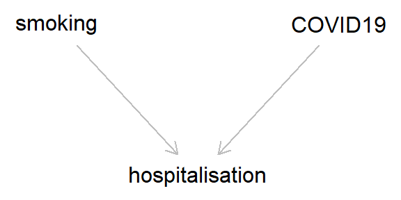
That is, if both smoking and COVID-19 cause hospitalisation, then, conditioning on being hospitalised, the relationship between smoking and COVID-19 is going to be biased. Even if the true association between smoking and COVID-19 is null, we would observe a negative association in this selected sample (and if smoking does increase the risk of COVID-19 - as is probable - then this risk will appear lower, or even reversed, in hospitalised patients). Here’s some code to illustrate this - Have a play around with the different parameters and see how the results change.

## Set seed
set.seed(987)

## Simulate smoking variable
smk <- rbinom(10000, size = 1, prob = 0.2)
table(smk)

## smk
##    0    1 
## 8005 1995

## Simulate COVID-19 variable ('log(1)' means that
## smoking does not cause COVID-19; increase this
## parameter to alter whether smoking causes COVID-19)
covid_p <- plogis(log(0.05) + (log(1) * smk))
covid <- rbinom(n = 10000, size = 1, prob = covid_p)
table(covid)

## covid
##    0    1 
## 9517  483

## Simulate hospitalisation (cause by both smoking
## and COVID-19)
hosp_p <- plogis(log(0.05) + (log(5) * smk)
                 + (log(5) * covid))
hosp <- rbinom(n = 10000, size = 1, prob = hosp_p)
table(hosp)

## hosp
##    0    1 
## 9137  863

## Unbiased/true association between smoking and COVID-19
mod_smk_true <- glm(covid ~ smk, family = "binomial")
exp(cbind(OR = coef(summary(mod_smk_true))[, 1], 
          confint(mod_smk_true))["smk", ])

##        OR     2.5 %    97.5 % 
## 0.9150688 0.7198269 1.1511484

## Biased association between smoking and COVID-19
## when conditioning on hospitalisation
mod_smk_bias <- glm(covid ~ smk, family = "binomial", 
            subset = hosp == 1)
exp(cbind(OR = coef(summary(mod_smk_bias))[, 1], 
          confint(mod_smk_bias))["smk", ])

##        OR     2.5 %    97.5 % 
## 0.5930030 0.4053150 0.8607785

Collider bias everywhere!

Once you know about collider bias it’s difficult not to see it everywhere, and the resulting creeping doubts may wreck all of your lovely conclusion. Collider bias is an ever-present threat to much observational research⁴, one which can be very difficult to detect or correct for.

So far in this blog we’ve only focused on the simplest examples of collider bias, where the exposure and outcome directly cause the collider. But there are more complex forms of collider bias, as well.

For instance, even if the outcome doesn’t cause the collider, but a different variable does, and this variable also causes the outcome, then this can result in collider bias. As an example, say we’re working with a prospective cohort study. Our exposure of interest is socioeconomic position, which causes continued study participation (higher SEP = greater chance of continued participation). And our outcome of interest is well-being (coded as a binary variable for simplicity). In this hypothetical example well-being doesn’t cause study participation, but age does cause both well-being and continued participation (see the DAG below for a clearer summary).

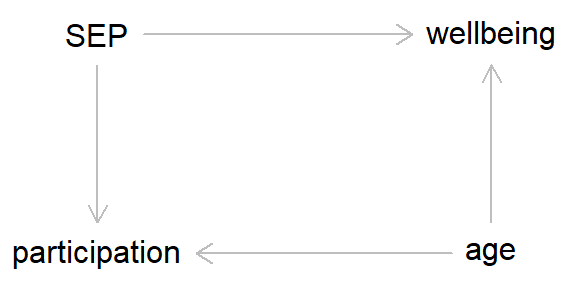
In this example, if there is missing data due to continued study participation, then unadjusted associations between SEP and wellbeing will be biased, as study participation is acting as a collider between the exposure and the outcome. However, if we adjust for ‘age’, then this breaks the path leading from ‘wellbeing’ to ‘participation’, meaning that we will now obtain an unbiased estimate of the SEP-wellbeing association.

Here’s some simulation code to demonstrate this, where the true odds ratio of SEP on well-being should be 5.⁵

## Set seed
set.seed(5678)

## Simulate SEP (caused by nothing; will treat as a
## binary variable here for simplicity; 1 = high SEP)
sep <- rbinom(10000, size = 1, prob = 0.5)
table(sep)

## sep
##    0    1 
## 5141 4859

## Simulate age (also caused by nothing)
age <- rnorm(10000, 50, sd = 10)
summary(age)

##    Min. 1st Qu.  Median    Mean 3rd Qu.    Max. 
##   14.89   43.13   49.76   49.89   56.58   84.66

## Simulate high well-being (caused by both SEP and age;
## higher SEP and age = greater well-being; again, using
## a binary variable just for simplicity)
wellbeing_p <- plogis(log(0.05) + (log(5) * sep) +
                  log(1.05) * age)
wellbeing <- rbinom(n = 10000, size = 1, prob = wellbeing_p)
table(wellbeing)

## wellbeing
##    0    1 
## 4507 5493

## Simulate study participation (also caused
## by both SEP and age - higher SEP and older
## age = greater study participation)
participation_p <- plogis(log(0.05) + (log(5) * sep)
                          + (log(1.05) * age))
participation <- rbinom(n = 10000, size = 1, 
                        prob = participation_p)
table(participation)

## participation
##    0    1 
## 4511 5489

## Biased association between SEP and well-being in selected
## sample if not adjust for age
mod_sep_bias <- glm(wellbeing ~ sep, family = "binomial",
                    subset = participation == 1)
exp(cbind(OR = coef(summary(mod_sep_bias))[, 1], 
          confint(mod_sep_bias))["sep", ])

##       OR    2.5 %   97.5 % 
## 4.352498 3.867086 4.902239

## Unbiased association between SEP and smoking in
## selected sample when adjust for age
mod_sep_unbias <- glm(wellbeing ~ sep + age, family = "binomial", 
                      subset = participation == 1)
exp(cbind(OR = coef(summary(mod_sep_unbias))[, 1], 
          confint(mod_sep_unbias))["sep", ])

##       OR    2.5 %   97.5 % 
## 5.042995 4.454530 5.715296

Another, slightly more complex, example of collider bias is known as ‘M-bias’ (because the DAG is ‘M’ shaped). Here, we are interested in estimating the causal effect of X on Y, and our three potential covariates are C1, C2 and C3. In this example, X does not cause Y, but C1 causes both X and C2, and C3 causes both Y and C2. From the DAG below it’s clear that C2 is acting as a collider, as the two arrows from C1 and C3 both project into - cause - C2.

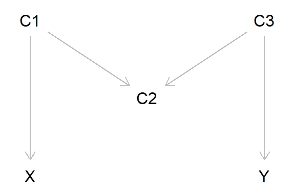
In this example, would we need to adjust for any of the potential covariates to get an unbiased estimate of the X-Y association? The answer is ‘no’. This is because as variable C2 is a collider, any information about X and Y via C1 and C3 gets ‘blocked’ by C2. If we were to adjust for C2 (or C2 represents study selection, so is implicitly conditioned upon), then we would get bias, as information can now ‘flow’ from X to Y via C1 and C3. If we also adjusted for C1 and/or C3, this would again block the flow of information, again resulting in a unbiased estimate.

This scenario is simulated below:

## Set seed
set.seed(98765)

## Simulate C1 (continuous; caused by nothing)
c1 <- rnorm(10000, mean = 0, sd = 1)
summary(c1)

##      Min.   1st Qu.    Median      Mean   3rd Qu.      Max. 
## -3.520305 -0.648206  0.004661  0.013996  0.699533  3.606542

## Simulate X (continuous; caused by C1)
x <- 0 + (0.5 * c1) + rnorm(10000, mean = 0, sd = 1)
summary(x)

##      Min.   1st Qu.    Median      Mean   3rd Qu.      Max. 
## -4.304194 -0.758166  0.003954  0.002740  0.753951  4.687440

## Simulate C3 (continuous; caused by nothing)
c3 <- rnorm(10000, mean = 0, sd = 1)
summary(c3)

##      Min.   1st Qu.    Median      Mean   3rd Qu.      Max. 
## -4.058914 -0.660036  0.007966 -0.000348  0.660825  4.219089

## Simulate Y (continuous; caused by C3)
y <- 0 + (0.5 * c3) + rnorm(10000, mean = 0, sd = 1)
summary(y)

##     Min.  1st Qu.   Median     Mean  3rd Qu.     Max. 
## -4.07183 -0.78688 -0.02655 -0.01581  0.74373  4.06271

## Simulate C2 (binary; caused C1 and C3)
c2_p <- plogis(log(1) + (log(3) * c1) 
               + (log(3) * c3))
c2 <- rbinom(n = 10000, size = 1, prob = c2_p)
table(c2)

## c2
##    0    1 
## 5016 4984

### Explore different models

## No adjustment for any covariates (no bias)
mod1 <- lm(y ~ x)
cbind(X = coef(summary(mod1))[, 1], 
          confint(mod1))["x",]

##            X        2.5 %       97.5 % 
##  0.009701162 -0.009898513  0.029300836

## Adjustment for C2 (bias, as adjusting for the
## collider C2; results in a negative association
## between X and Y)
mod2 <- lm(y ~ x + c2)
cbind(X = coef(summary(mod2))[, 1], 
      confint(mod2))["x",]

##            X        2.5 %       97.5 % 
## -0.024890632 -0.044598061 -0.005183203

## Implicitly conditioning on C2 (e.g., due
## to selection/missing data; bias)
mod3 <- lm(y ~ x, subset = c2 == 1)
cbind(X = coef(summary(mod3))[, 1], 
      confint(mod3))["x",]

##           X       2.5 %      97.5 % 
## -0.01559853 -0.04381297  0.01261590

## Adjustment for C1 and C2 (no bias, as 
## adjusting for  C1 blocks the effect of
## adjusting for the collider C2)
mod4 <- lm(y ~ x + c1 + c2)
cbind(X = coef(summary(mod4))[, 1], 
      confint(mod4))["x",]

##            X        2.5 %       97.5 % 
## -0.001749532 -0.023406548  0.019907484

## Adjustment for C3 and C2 (no bias, as 
## adjusting for  C3 blocks the effect of
## adjusting for the collider C2)
mod5 <- lm(y ~ x + c3 + c2)
cbind(X = coef(summary(mod5))[, 1], 
      confint(mod5))["x",]

##            X        2.5 %       97.5 % 
##  0.010454077 -0.007421993  0.028330148

## Adjustment for C1, C3 and C2 (no bias, as 
## adjusting for both C1 and C3 blocks the 
## effect of adjusting for the collider C2)
mod6 <- lm(y ~ x + c1 + c3 + c2)
cbind(X = coef(summary(mod6))[, 1], 
      confint(mod6))["x",]

##            X        2.5 %       97.5 % 
##  0.006803969 -0.012801595  0.026409533

This section has shown that collider bias can occur not just when the exposure and outcome cause the collider, but also when factors relating to the exposure and outcome also cause a collider - Hence the definition above that collider bias occurs “when one conditions on a common consequence of (i.e., a variable caused by) the exposure and outcome (or factors related to the exposure and outcome)”.

These examples have also demonstrated that adjusting for all known covariates isn’t always a good idea, especially when some of those variables are colliders. This may result in more bias that not adjusting for said covariates. For instance, in the ‘M-bias’ example, if C2 was measured/observed but C1 and C3 were unmeasured/unobserved, adjusting for C2 would result in bias while not adjusting for it would not. For estimating causal effects, the causal relations between variables has to be taken into consideration, as this will determine the parameters to include in a model; and you may not have to adjust for some - or even all - variables. Sometimes less really is more.

How to avoid collider bias

Avoiding collider bias can be difficult, as it is often tricky to diagnose, requires knowing the causal relations between variables, and the impact of collider bias depends on the strength of those causal effects. Often these causal relations, and their magnitude, are unknown, and can only be dimly estimated. Still, being aware of collider bias is an important first step toward enlightenment, and here are a few suggestions to try and mitigate the evils of collider bias.

• Use DAGs! As I’ve reiterated throughout these blogs, making a DAG is an important first step of many analyses. Even if the causal relations aren’t known with certainty, it is often still possible to make informed decisions about these effects. Even a DAG based on hypothesised relations and imperfect information is better than no DAG, as it makes your assumptions clear to others. From said DAG, it should be possible to identify whether any variables are acting as colliders and what can be done to try and mitigate this potential bias.

• If you do spot any collider variables in your DAG, don’t adjust for them in your model. If adjusting for a collider is unavoidable, try to block their path to avoid bias (as we showed with the ‘M-bias’ example above).

• Avoiding collider bias can be more challenging if the collider is implicit (e.g., conditioning on study participation/missing data). In these cases, sometimes adjusting for additional covariates can remove bias - as with the example of SEP and well-being, above - but may require a more advanced approach. Some methods to quantitatively explore and account for potential collider bias include: the AscRtain R package, multiple imputation, inverse-probability weighting, plus many others.

• Perhaps most importantly, at the study design stage try and ensure that the sample is representative of target population, thereby avoiding issues of selection bias altogether (this is easier said than done, though, as random sampling is notoriously difficult; and even if the initial sample is random, if the study is longitudinal non-random drop-out over time may result in bias. Still, it’s generally better to try and get a random sample initially than to worry about collider bias at the analysis stage where it may be too late…).

Summary

Okay, this post has started to shade into missing data territory now, which is a huge and complex topic in itself⁶, so I’ll end this intro to collider bias here. This post has covered:

• What collider bias is
• How to spot colliders in DAGs
• How (and why) collider bias can bias inferences
• A brief introduction on how to avoid or overcome collider bias

In the next post, I’ll introduce the third ‘epidemiological horseman of the apocalypse’ (after ‘confounding bias’ and ‘collider bias’): measurement bias.

Further reading

In recent years awareness of collider bias has increased substantially. Some key introductory texts are:

• Judea Pearl and Dana Mackenzie’s Book of Why is a gentle introduction to causal inference, including collider bias (especially chapters 3, 5 and 6).
• Chapter 8 of Miguel Hernán and Jamie Robins’ book Causal Inference: What If is a great and more detailed introduction to collider/selection bias.
• This paper on collider bias in COVID-19 research by Gareth Griffith and colleagues is also a nice explanation of collider bias and how it can result in misleading conclusions (see also this summary paper the MRC-IEU blogs here and here.
• Marcus Munafó and colleagues also have a fab intro paper to collider bias, with the great title ‘collider scope’. The example of the coin toss and bell-ringing is taken from this paper.

Stata code

*** Acting skill, attractiveness and fame example

* Clear data, set observations and set seed
clear
set obs 10000
set seed 54321

* Simulate 'acting skill'
gen skill = rnormal(0, 1)
sum skill

* Simulate attractiveness (again, caused by age)
gen attract = rnormal(0, 1)
sum attract

* And now simulate 'becoming famous' (caused
* by both skill and attractiveness)
gen famous_p = invlogit(log(0.05) + (log(5) * skill) /// 
    + (log(5) * attract))
gen famous = rbinomial(1, famous_p)
tab famous

* Show that skill and attractiveness are independent, 
* if not condition on 'fame'
regress attract skill

* Now include 'famous' in this model, to show this
* biases the 'skill-attractiveness' relationship
regress attract skill famous

* Similar to above, but now conditioning on 'famous'
* by only including famous == 1 in the model
regress attract skill if famous == 1

* Show this in a plot
twoway (scatter attract skill if famous == 1, ///
                mcol(red%30) msize(1)) ///
    (scatter attract skill if famous == 0, ///
            mcol(black%30) msize(1)) ///
    (lfit attract skill if famous == 1, ///
            lcol(red) lwidth(1)) ///
    (lfit attract skill, lcol(blue) lwidth(1)), ///
    legend(lab(1 "Famous") lab(2 "Not famous") ///
            lab(3 "Famous sub-sample") ///
        lab(4 "Whole sample"))
        
* And now model conditioning on not being famous
regress attract skill if famous == 0


*** Smoking, COVID-19 and hospitalisation example

* Clear data, set observations and set seed
clear
set obs 10000
set seed 987

* Simulate smoking variable
gen smk = rbinomial(1, 0.2)
tab smk

* Simulate COVID-19 variable ('log(1)' means that
* smoking does not cause COVID-19; increase this
* parameter to alter whether smoking causes COVID-19)
gen covid_p = invlogit(log(0.05) + (log(1) * smk))
gen covid = rbinomial(1, covid_p)
tab covid

* Simulate hospitalisation (cause by both smoking
* and COVID-19)
gen hosp_p = invlogit(log(0.05) + (log(5) * smk) ///
    + (log(5) * covid))
gen hosp = rbinomial(1, hosp_p)
tab hosp

* Unbiased/true association between smoking and COVID-19
logistic covid smk

* Biased association between smoking and COVID-19
* when conditioning on hospitalisation
logistic covid smk hosp


*** SEP, well-being and study drop-out example 
*** (well-being not cause drop-out, but is 
*** associated with 'age', which does)

* Clear data, set observations and set seed
clear
set obs 10000
set seed 5678

* Simulate SEP (caused by nothing; will treat as a
* binary variable here for simplicity; 1 = high SEP)
gen sep = rbinomial(1, 0.5)
tab sep

* Simulate age (also caused by nothing)
gen age = rnormal(50, 10)
sum age

* Simulate high well-being (caused by both SEP and age;
* higher SEP and age = greater well-being; again, using
* a binary variable just for simplicity)
gen wellbeing_p = invlogit(log(0.05) + (log(5) * sep) ///
    + log(1.05) * age)
gen wellbeing = rbinomial(1, wellbeing_p)
tab wellbeing

* Simulate study participation (also caused
* by both SEP and age - higher SEP and older
* age = greater study participation)
gen part_p = invlogit(log(0.05) + (log(5) * sep) ///
    + (log(1.05) * age))
gen participation = rbinomial(1, part_p)
tab participation

* Biased association between SEP and well-being in selected
* sample if not adjust for age
logistic wellbeing sep if participation == 1

* Unbiased association between SEP and smoking in
* selected sample when adjust for age
logistic wellbeing sep age if participation == 1


*** M-bias example

* Clear data, set observations and set seed
clear
set obs 10000
set seed 98765

* Simulate C1 (continuous; caused by nothing)
gen c1 = rnormal(0, 1)
sum c1

* Simulate X (continuous; caused by C1)
gen x = 0 + (0.5 * c1) + rnormal(0, 1)
sum x

* Simulate C3 (continuous; caused by nothing)
gen c3 = rnormal(0, 1)
sum c3

* Simulate Y (continuous; caused by C3)
gen y = 0 + (0.5 * c3) + rnormal(0, 1)
sum y

* Simulate C2 (binary; caused C1 and C3)
gen c2_p = invlogit(log(1) + (log(3) * c1) ///
    + (log(3) * c3))
gen c2 = rbinomial(1, c2_p)
tab c2


** Explore different models

* No adjustment for any covariates (no bias)
regress y x

* Adjustment for C2 (bias, as adjusting for the
* collider C2; results in a negative association
* between X and Y)
regress y x c2

* Implicitly conditioning on C2 (e.g., due
* to selection/missing data; bias)
regress y x if c2 == 1

* Adjustment for C1 and C2 (no bias, as 
* adjusting for the C1 blocks the effect of
* adjusting for the collider C2)
regress y x c1 c2

* Adjustment for C3 and C2 (no bias, as 
* adjusting for the C3 blocks the effect of
* adjusting for the collider C2)
regress y x c2 c3

* Adjustment for C1, C3 and C2 (no bias, as 
* adjusting for both C1 and C3 blocks the 
* effect of adjusting for the collider C2)
regress y x c1 c2 c3