Dagatha Christie and the Conundrum of Causality (1)

Dagatha sits beside a fire in her armchair, with her labradoodles Hernan, Robins and Pearl dozing around her feet. She reads a letter from a fellow named Bennett asking for her advice: Dagatha being known in these parts as an expert in such matters. Bennett writes that when he was ill his friends prayed for him and - lo and behold - he got better. He asks Dagatha whether it is possible that their prayers caused him to recover. He knows that the drugs and medical attention helped (plus simply recovering naturally/regression to the mean), but believes that their prayers might have had an effect in addition to these more obvious explanations. After all, when they prayed, he did get better!

Dagatha responds by saying that, as Bennett rightly points out, his friends’ prayers occurred at the same time as these other factors shaping his recovery, meaning that it is difficult to know the causal effect of prayer on recovery based on this one experience. However, given what we know about the laws of physics it is unlikely that their prayers had a causal effect on his recovery. Still, as there is probably no harm to Bennett’s friends prayers (as long as he isn’t using prayer in lieu of traditional medical treatment!), Dagatha suggests that his friends could continue their behaviour if it makes them feel like they’re helping - It probably makes Bennett’s friends feel better and, who knows, perhaps if Bennett knows that his friends are praying for them it might help his recovery.

This simple example - although unlikely to win any literary awards - raises some interesting issues regarding the nature of causality¹. The aim of this post is to starting thinking about these issues, and the wider concept of causal inference, in a gentle introductory manner. Later posts will expand on these themes, exploring how and when we can infer causality from research, and introducing concepts such as confounding, mediation and collider/selection bias. I will focus on using simulated data to explore and understand these ideas from a causal perspective as I’m not a particularly ‘mathematical’ thinker and simulating data often helps me understand these ideas more clearly than formal proofs or equations.

Although causality is central to the application of science - after all, why adopt an intervention if you’re not even sure the intervention actually causes the desired response? - in our training as science students these issues are often overlooked. That’s my experience, at least (I have a background in psychology and anthropology). It was only when I joined the epidemiology department at the University of Bristol a few years ago that causality was really taken seriously. After I took these issues on board my approach to research changed, with a focus on being clear of the aims of the research (descriptive/associational vs predictive vs causal) and, if causal, defining the causal question carefully and as clearly as possible using causal graphs to make these assumptions clear (both to myself and to readers). Hopefully this ‘causal revolution’ will continue to spread and find its way into more people’s research. I believe this will improve science for the better.

But I’m getting ahead of myself here. First of all, we need a working definition of causality and a causal model of how (we think) the world works.

Defining causality

Beyond the classic ‘correlation does not equal causation’ dictum, what causation actually is is often left rather vague (in some cases - and given certain assumptions - we will see that correlation can equal causation; indeed, causation without correlation is impossible). In 1748 the philosopher David Hume gave an early definition of causality (although in reality it is two definitions smooshed together):

“We may define a cause to be an object followed by another, and where all the objects, similar to the first, are followed by objects similar to the second. Or, in other words, where, if the first object had not been, the second never had existed.”

In this somewhat-tortured prose, the first sentence defines causality in terms of a temporal sequence: y follows x, and hence x caused y. Although intuitively appealing, this doesn’t necessarily capture a causal relationship. Let’s take the example of Bennett’s friends prayers. If Bennett’s friends always prays when he gets ill, then we would always observe a strong association between prayer and recovery. However, this doesn’t mean that Bennett’s friends praying caused him to recover.

The second sentence of Hume’s definition is much closer to our current conceptions of causality; that is, in terms of interventions or counterfactuals. Here, rather than defining causality based on temporal sequences of observed data, we ask what would happen to y if we change x? To answer this question we must alter x - holding everything else equal - to see whether y changes; if so, then we can say that x causes y. To return to the prayer example, from this perspective causality can be inferred if we intervene on Bennett’s friends praying (say, only praying half of the time) and find a difference in his recovery outcomes between the two conditions².

Representing causality

Now that we have a definition of causality, our next concern is how to represent this causal structure. This is where Directed Acyclic Graphs (DAGs; also known as ‘causal graphs’) come in. The name is a bit of a mouthful, but the rationale behind them is quite simple: to represent our causal knowledge (or causal assumptions) about the world. Once understood, I have found them to be a powerful tool when thinking about research questions and designing my analyses.

Let’s break down each component of ‘Directed Acyclic Graph’:

Directed: This means that causality only ‘flows’ in one direction. That is, if variable x causes variable y, y cannot also cause x³.
Acyclic: There are no loops/cycles in the DAG, meaning that a variable cannot cause itself. E.g., you cannot have a DAG where x causes y, y causes z and then z causes x.
Graph: In mathematics, ‘graphs’ refer to nodes joined by edges to model relations between objects. In DAGs, ‘nodes’ are variables and ‘edges’ are one-directional arrows denoting causal relationships.

Okay, with that rather theoretical background out the way, we’ll build our first DAG!⁴

Building a DAG

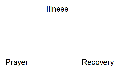
The above probably all sounds rather abstract, but making a DAG basically just consists of drawing arrows between variables. The first thing we need to do is specify our variables (the nodes of the DAG). Using the prayer example again, these three nodes are illness, prayer and recovery, like so:

Next, we add the arrows (edges) denoting causal relationships. Both Dagatha and Bennett agree that Bennett’s illness causes his friends to pray for him, and that illness also causes recovery (the intermediate step between ‘illness’ and ‘recovery’ of taking drugs/seeing a Dr isn’t displayed in this DAG, to keep things simple). So we can add those arrows in:

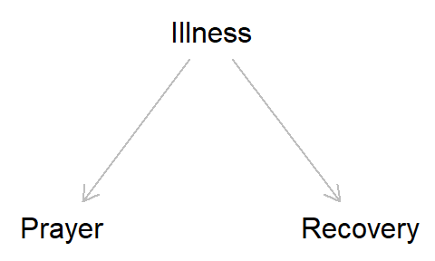
Because illness causes both prayer and recovery, we can now see why prayer and recovery are related in the observed data, even if the relationship is not causal. This is because even though causation is one-directional, associations can flow either way. Even though we know that illness must cause recovery (because the reverse is impossible), a regression/correlation/chi-square test/etc. can’t know this, and will find an association of illness predicting recovery as readily as it will on recovery predicting illness. Put another way, standard statistical analyses are blind to causality, and can only detect associations; whether we interpret these relationships as causal depends on our knowledge/assumptions of the underlying system.

Because of this property, unadjusted models of the association between prayer and recovery will be biased (i.e., not the true causal value). When the exposure (or independent variable, or predictor variable) and the outcome (or dependent variable, or response variable) are both caused by a third variable, we say that the exposure-outcome relationship is confounded. We can remove this bias from confounding by adjusting for, or stratifying by, ‘illness’ in our statistical models to close this previously-open ‘back-door path’, resulting in accurately estimating the causal effect between prayer and recovery. But we’re getting ahead of ourselves again here (more on confounding in a future post).

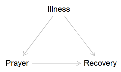
Getting back to our main topic here of constructing DAGs, where Dagatha and Bennett diverge is the causal relationship between ‘prayer’ and ‘recovery’; Dagatha believes that there is no causal relationship between ‘prayer’ and ‘recovery’ (i.e., no arrow, as in the DAG above), while Bennett believes that there might be a causal relationship between prayer and recovery (as in the DAG below). These two DAGs represent different causal hypotheses about the world, and by drawing them we can clearly see where Dagatha and Bennett differ in their causal assumptions.

Summary

Hopefully this has been a gentle introduction to DAGs and causality. The key take-home messages are that: 1) Causality is defined in terms of interventions/counterfactuals; and 2) We can use DAGs to represent our causal assumptions about the world.

This has - I hope! - been relatively simple and all a bit, well, obvious. So obvious, in fact, that you might be wondering what all the fuss is about with DAGs and causality. While we are starting with incredibly simple examples, the concepts that we’re building up will get increasingly complex and I hope all this simple foundational work will pay dividends once we reach these more complicated examples. Once we start looking at these complex cases involving more covariates, mediators, colliders and selection, a causal approach using DAGs will hopefully provide more clarity than a non-causal/non-DAG approach.

Here is a bullet point summary of DAGs and answers to some frequently asked questions:

In a DAG, the nodes represent variables and the arrows represent causal relationships between these variables.
Even though causality can only run in one direction, associations can ‘flow’ in either direction, meaning that statistical tests cannot determine causality; additional assumptions outside the statistical model are needed to infer causality.
No arrow means no causality. This doesn’t mean that there will be no association between two variables which are not causally related, however. As we saw above, prayer and recovery can still be associated (via illness), even if prayer does not cause recovery.
Depending on the aims of our research, we do not need to represent every step in the causal chain in a DAG. E.g., illness causes recovery through seeking medical attention, but we don’t need to represent ‘seeking medical attention’ as a node on the DAG if we are just interested in the causal relationship between illness and recovery.
The causal arrows can either be deterministic (i.e., x always causes y) or probabilistic (i.e., x sometimes, although not always, causes y). In real-life most causal relationships are probabilistic, rather than deterministic. Think of smoking and lung cancer; smoking causes lung cancer, but not everyone who smokes will get lung cancer.
The causal arrows do not denote the form of the relationship (that is, the causal relationships are non-parametric). They can be between continuous, binary, categorical, etc. variables, and the relationship could be linear or non-linear. Arrows also do not specify whether the relationship is positive or negative, or the magnitude of the association. A causal arrow simply says that x causes y, nothing more.

In the next post, I will describe methods for simulating data based on a DAG, which we will use throughout later posts to explore confounding, mediation, colliders and so on. As this website is built using R, the main scripts will be in R coding language; but as I also frequently work in Stata I will also present the code in Stata format as well.

And if you’re wondering who is correct - Dagatha or Bennett - based on a cochrane systematic review and meta-analysis of randomised-controlled trials, it would appear that anonymous prayer has no discernible impact on health outcomes. It is possible that by telling someone that you’re praying for them this might alter their recovery, although there has been much less research on this (and, interestingly, one study found an increased risk of complications after surgery among those who knew they were being prayed for). So it would appear that Dagatha was correct, at least in terms of anonymous prayers.

Coda: Modeling reciprocal causation using DAGS

As discussed above, reciprocal causation between variables is verboten in DAGs. But there are methods to get around this, which is handy as many phenomena of interest are likely to display such reciprocal relationships. Let’s take weight and exercise as our exposures, and cardiovascular health as our outcome. Say that weight causes exercise (with increased weight causing lower rates of exercise), but exercise also causes people to change their weight (with more exercise causing weight loss), and both impact cardiovascular health (with higher weight and less exercise causing greater risk of cardiovascular disease; CVD).

Intuitively, we might draw a DAG like this, with a double-headed arrow between weight and exercise:

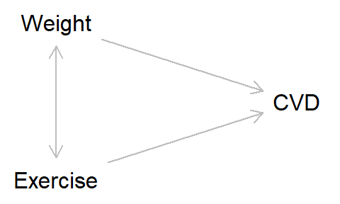
However, this breaks the rules of DAGs, as the causal arrows are now no longer one-directional. Instead, we can split weight and exercise into different time-points and represent the causal relationships this way. That is, weight at time 1 causes both weight at time 2 and exercise at time 2, while exercise at time 1 causes both exercise at time 2 and weight at time 2, and so on. The DAG will look a little like this:

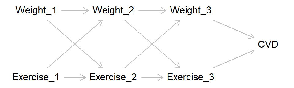
This starts getting to the territory of time-varying covariates, which are a bit advanced for our purposes here, but hopefully this gives a flavour of how reciprocal causation and time-varying effects can be represented using DAGs.