The next letter Dagatha receives is from a frantic man called Gary who starts with the rather arresting opening salvo: “AM I GOING TO DIE FROM COVID BECAUSE I’M BALD?!?!”. Calming down slightly, Gary goes on to explain that COVID-19 may impact bald people - like himself - more severely than the rest of the population, or so he read in some newspapers1. This is based on scientific research published by legitimate scientists in peer-reviewed journals, and with a plausible-sounding theory regarding androgens which may affect both hair loss and immune function. Can Dagatha help Gary here? It’s not clear to Gary why hair loss would be linked to more serious COVID symptoms, but if it’s published science can it be that wrong?
Dagatha peruses some of these research papers to take a look for herself2. These studies looked at small numbers of Spanish patients hospitalised with severe COVID-19 symptoms, and then compared the proportion of those patients with hair loss to population-level hair loss statistics. They apparently found that there were more people with hair loss hospitalised with COVID than would be expected based on these wider statistics, and concluded that androgens - as proxied by hair loss - may increase the risk of severe COVID-19. However, Dagatha is suspicious that this association may be spurious, and caused by not properly accounting for age differences3; as age is associated with both baldness and COVID-19 severity, it’s plausible - and indeed quite likely - that the supposed associations between hair loss and COVID severity are explained by age differences, not baldness4.
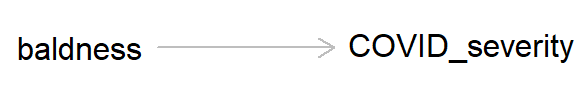
So other than maybe breathing a little easier if you have hair loss, what’s the message of this preamble? This example is a classic case of confounding, where a lurking ‘third variable’ can bias an association between two variables. As always, we can draw a DAG to represent the causal hypothesis of the researchers who claim that hair loss - which in this case is used as a proxy for androgen activity - may cause more severe COVID-19 symptoms.
But if we add ‘age’ into this DAG, we can see how age, by causing both baldness and COVID severity, can act as a ‘back-door path’ by which associations can flow from baldness to COVID severity, even if in reality hair loss has no causal effect on COVID-19 severity.
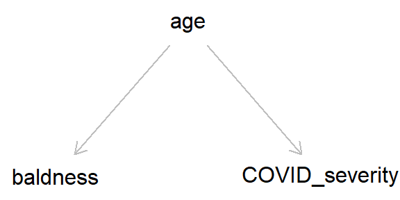
As we went through in the last post, by simulating data we can get a better idea of how these different causal structures impact our inferences. So let’s simulate the DAG above, where age causes both baldness and COVID-19 severity (hospitalisation with COVID-19), while baldness has no causal effect on hospitalisation (Stata code is provided at the end of the post).
## Set the seed so data is reproducible
set.seed(9876)

## Simualate age (caused by nothing)
age <- rnorm(n = 10000, mean = 50, sd = 10)

## Simulate baldness (caused by age)
# Need to create probabilities from the logit scale
# first, then sample from that (here, we're saying
# that a one-unit increase in age causes a 7%
# increase in the odds of having hair loss)
baldness_p <- plogis(log(0.05) + (log(1.07) * age))
baldness <- rbinom(n = 10000, size = 1, prob = baldness_p)
table(baldness)
## baldness
## 0 1
## 4075 5925## And now simulate hospitalisation with
## COVID-19 (COVID severity; caused by age)
# Here, the probability of having severe COVID is rare,
# but that it increases with age (by 5% odds per year)
severity_p <- plogis(log(0.005) + (log(1.05) * age))
severity <- rbinom(n = 10000, size = 1, prob = severity_p)
table(severity)## severity
## 0 1
## 9418 582Now, as we had complete control over how the data were generated, we know that there is no causal effect of baldness on COVID-19 severity. But if we run a simple univariable logistic regression model of baldness on severity, we see an association between the two. If we took this model at face value as a causal effect, we would say that baldness causes a 30% increase in the odds of having severe COVID-19. For a more intuitive summary of this result, we can look at the predicted probabilities of having severe COVID in each category of ‘baldness’; here, we can see that people without hair loss have a 5% chance of being hospitalised with COVID, while this increases to 6.4% in the group with hair loss.
mod_noAge <- glm(severity ~ baldness, family = "binomial")

# Summary on the odds ratio scale
exp(cbind(OR = coef(summary(mod_noAge))[, 1],
          confint(mod_noAge)))
## OR 2.5 % 97.5 %
## (Intercept) 0.05269956 0.0456389 0.06049113
## baldness 1.29308369 1.0866992 1.54287369# Look at predicted probabilities for each category of
# baldness (create a new data frame then use the
# 'predict' command)
newdata <- data.frame(baldness = c(0, 1))
newdata$probs <- predict(mod_noAge, newdata = newdata,
type = "response")
newdata## baldness probs
## 1 0 0.05006135
## 2 1 0.06379747Hopefully this makes it clear how confounding variables can lead to bias in our causal estimates. But how do we remove this bias to obtain a ‘true’ estimate?5 Going back to our analogy of information ‘flowing’ through DAGs regardless of the direction of causality, if we adjust for (or control for, or stratify by) age, we can stop the information flowing between baldness and COVID severity. We can do this by simply adding ‘age’ as a covariate in our regression model, like so:
mod_age <- glm(severity ~ baldness + age,
               family = "binomial")

# Summary on the odds ratio scale
exp(cbind(OR = coef(summary(mod_age))[, 1],
          confint(mod_age)))
## OR 2.5 % 97.5 %
## (Intercept) 0.005415179 0.003394018 0.00857251
## baldness 0.962206283 0.800846775 1.15864508
## age 1.048519540 1.039308942 1.05785102# Look at predicted probabilities for each category of
# baldness at different values of age
newdata <- data.frame(age = rep(c(30, 50, 70), each = 2),
baldness = rep(c(0, 1), 3))
newdata$probs <- predict(mod_age, newdata = newdata,
type = "response")
newdata## age baldness probs
## 1 30 0 0.02194186
## 2 30 1 0.02113011
## 3 50 0 0.05470257
## 4 50 1 0.05274420
## 5 70 0 0.12988174
## 6 70 1 0.12558951Now we can see that there is a strong effect of age on COVID-19 severity and no effect of baldness. And looking at the predicted probabilities of hospitalisation by baldness stratified by age, we see that the probabilities are equal within each age.
Defining confounding
The example above has shown us how confounding can bias associations and how to remove this bias, but how can we actually define confounding? Prior to the rise of causal inference, an agreed-upon definition had proven surprisingly elusive.
Some common definitions include “any variable that is correlated with both x and y” or “if including a variable in a model alters the association between x and y, then that’s a confounder”6. These approaches would seem to make sense for our example above, as age is correlated with both baldness and COVID severity - and adjusting for it alters the association between the two - so would therefore be seen as a confounder. But consider the DAG below:

Here, we’re interested in the causal effect of diet on cardiovascular disease (CVD). In this scenario, diet does not cause CVD directly, but causes CVD indirectly through its effect on hypertension (that is, diet causes hypertension, which in turn causes CVD). In this example, even though hypertension is associated with both diet and CVD, treating it as a confounder and adjusting for it in a regression model would be nonsensical, as by controlling for hypertension we’re completely blocking the path by which diet causes CVD!7 The point is that hypertension in this example fits both definitions of confounding given above, yet clearly controlling for this variable would be a huge mistake.
Taking a causal perspective, we can define a confounder quite simply as “a variable which causes x and y”.8 This might still sound a bit abstract, but simple cases of confounding can quite easily be spotted in DAGs as a causal arrow from one variable which causes both x and y. The example of age confounding baldness and COVID-19 severity (repeated below) is a canonical example of confounding.

Fortunately, as we’ve seen above, assuming that the confounders are known and measured it is relatively easy to remove bias due to confounding: simply adjust for the confounding variables in your model.
Here’s a slightly more complicated example:

Here we’re interested in estimating the causal relationship between smoking and lung cancer. Age is a confounder which causes lung cancer directly, and also causes smoking indirectly through attitudes towards the health risks of smoking: age therefore causes both smoking and lung cancer. But now take attitudes. Attitudes causes smoking, but it doesn’t cause lung cancer through any other route. However, even though attitudes isn’t technically a confounder because it doesn’t cause x and y, it can still be considered a surrogate confounder because it is associated with age, which in turn causes lung cancer; so if age was not measured in this study for some reason, then adjusting for attitudes should still return an unbiased estimate because it blocks the back-door path leading from smoking to lung cancer via attitudes and age.
Given this situation, we can either adjust for age or attitudes and this will return an unbiased causal effect of smoking on lung cancer. Let’s test this out with some simulated data:
## Set the seed so data is reproducible
set.seed(6789)

## Simualate age (caused by nothing)
age <- rnorm(n = 10000, mean = 50, sd = 10)

## Simulate attitudes (caused by age)
# Will say this is a normally-distributed variable
# with a mean of 0, and that older people have a
# more positive attitude towards smoking
attitudes <- -5 + (0.1 * age) +
  rnorm(n = 10000, mean = 0, sd = 1)
summary(attitudes)
## Min. 1st Qu. Median Mean 3rd Qu. Max.
## -5.221396 -0.965175 -0.024165 -0.007261 0.949688 5.447796## Simulate binary smoking variable (caused by
## attitudes)
smk_p <- plogis(log(0.2) + (log(2) * attitudes))
smk <- rbinom(n = 10000, size = 1, prob = smk_p)
table(smk)## smk
## 0 1
## 7909 2091## And now simulate lung cancer (caused by age
## and smoking)
lung_p <- plogis(log(0.005) + (log(1.05) * age) +
(log(5) * smk))
lung <- rbinom(n = 10000, size = 1, prob = lung_p)
table(lung)## lung
## 0 1
## 8987 1013Next, we can look at the unadjusted association between smoking and lung cancer - We know this will be biased because we haven’t adjusted for age or attitudes. As such, the odds ratio is approximately 6, even though we only simulated it to be 5.
mod_unadj <- glm(lung ~ smk,
               family = "binomial")

# Summary on the odds ratio scale
exp(cbind(OR = coef(summary(mod_unadj))[, 1],
          confint(mod_unadj)))
## OR 2.5 % 97.5 %
## (Intercept) 0.06061419 0.05504944 0.06656377
## smk 6.04918879 5.28374110 6.92947684Now we’ll adjust for age, a confounder which causes both smoking and lung cancer. Now the odds ratio is pretty much 5 (and the 95% confidence intervals contain this value), just as we simulated.
mod_age <- glm(lung ~ smk + age,
               family = "binomial")

# Summary on the odds ratio scale
exp(cbind(OR = coef(summary(mod_age))[, 1],
          confint(mod_age)))
## OR 2.5 % 97.5 %
## (Intercept) 0.006254198 0.004213855 0.009220302
## smk 4.729085728 4.107599187 5.446770256
## age 1.046053559 1.038506924 1.053711723We also could have adjusted for attitudes. Even though it only causes smoking, because it is associated with a factor (age) which does cause lung cancer, adjusting for ‘attitudes’ blocks this back-door path and again gives us an unbiased estimate of an odds ratio of 5 for smoking.
mod_att <- glm(lung ~ smk + attitudes,
               family = "binomial")

# Summary on the odds ratio scale
exp(cbind(OR = coef(summary(mod_att))[, 1],
          confint(mod_att)))
## OR 2.5 % 97.5 %
## (Intercept) 0.06183367 0.05613699 0.067927
## smk 4.66182713 4.02515802 5.402029
## attitudes 1.25251789 1.18924802 1.319501There is also no harm in adjusting for both age and attitudes, as it will give us an unbiased estimate of the effect of smoking on lung cancer, although really there is no need to adjust for both; adjusting for one variable closes the back-door path for both. Either way, we still get an odds ratio of 5.
mod_ageAtt <- glm(lung ~ smk + age + attitudes,
               family = "binomial")

# Summary on the odds ratio scale
exp(cbind(OR = coef(summary(mod_ageAtt))[, 1],
          confint(mod_ageAtt)))
## OR 2.5 % 97.5 %
## (Intercept) 0.006481207 0.003842316 0.01085727
## smk 4.706667844 4.059389900 5.46017281
## age 1.045327825 1.035111967 1.05570383
## attitudes 1.007428215 0.938451767 1.08145682Benefits of a causal approach to confounding
So what are the benefits of this causal approach to confounding? In my humble opinion there are a fair few, including:
- It provides a clear and unambiguous (and correct!) definition of what ‘confounding’ actually is. This has settled years of debate on how best to define confounding; turns out this is an impossible task without adopting a causal approach.
- As a result of this clear definition, it provides clarity on how to spot and adjust for confounding. This can really help when deciding which variables to include as potential covariates in your model. It also adds some discipline and thought to the process of variable selection, rather than the traditional ‘causal salad’ approach in which everything is just thrown into a regression without considering the causal structure of the data. It also means that you don’t have to adjust for variables which either have no relation to x or y, only cause x, or only cause y9.
- This approach makes it clear that in order to identify confounding - and make causal inferences more generally - you have to go beyond the model/data and bring in causal assumptions. This again highlights the importance of taking a causal approach seriously.
- It shows that, given the assumption that all confounders have been measured and controlled for, you can - tentatively at least - make causal claims from observational data. If you truly have captured all variables which confound the association between x and y, then what remains should be a causal estimate of this effect. We can therefore go beyond ‘correlation does not imply causation’ to say when correlation may in fact imply causation.
Not too shabby, eh?? So that’s confounding cracked, and we can now go about adjusting for confounding properly and making all kinds of causal claims from observational data, right? Alas, unfortunately things are never quite that simple.
In reality we:
- May not have recognised, controlled for or measured all possible confounders (more on this below)
- May not have measured the confounder well enough, leading to measurement error which could bias our results (more on measurement error in a later post)
- Might be unsure whether a variable is a confounder or a mediator; if the latter, then - as we saw briefly above - adjusting for a mediating variable will not return an unbiased causal estimate (more on this in the next post)10.
The curse of unmeasured confounding
One major issue with making causal claims from observational research is the possibility of there being additional confounders that we have either not measured in our study or that we didn’t even know existed. Take a longitudinal cohort study looking at the association between intake of a certain nutrient (say, beta-carotene) and some health outcome (say, mortality from cardiovascular disease [CVD]). At baseline, this study assessed diet/nutrient intake, in addition to a whole host of potential confounders (age, sex, socioeconomic position, exercise, etc.); participants were then followed for 10 years to see who died from CVD and whether this was associated with beta-carotene intake, controlling for all confounders mentioned above.
After 10 years, the researchers finally analysed the data and - success! - they find a strong association between beta-carotene intake and lower mortality from CVD. They eagerly write up their results in a paper and claim a causal link between beta-carotene consumption and reduced cardiovascular mortality; after all, they followed the causal recommendations above and adjusted for all possible confounders that they could think of. Additionally, while writing up the results a different team of scientists published an identical result from a different cohort study finding a protective effect of beta-carotene on cardiovascular mortality; the original team feel slightly irked that their big finding has been scooped, but feel even bolder about making causal claims as their finding has been independently replicated.
Randomised-controlled trials (RCTs) are then conducted to definitively test whether beta-carotene intake reduces mortality from CVD. However, once these RCT results are in they actually find that beta-carotene increases mortality from CVD, rather than reduces it. What the frig is going on here??11
The answer is unmeasured confounding. That is, despite the authors’ best efforts, there were still other factors associated with both the exposure (beta-carotene intake) and the outcome (mortality from cardiovascular disease) which confounded and biased this relationship. This is variable U in the DAG below.

Unfortunately this risk of unmeasured confounding is always a possibility in observational research, hence why it’s difficult to make definitive causal claims from this type of work. Any causal interpretation from observational research is therefore always subject to the impossible-to-prove assumption of ‘no unmeasured confounding’. In this example, the unmeasured confounder could be something like a ‘healthy lifestyle’, which is difficult to measure but may confound both diet and CVD mortality risk.
This then begs the question of why we should believe the RCT over the observational study? Random allocation to condition (receiving beta-carotene or not) means that there is no possibility of confounding, hence why RCTs are the ‘gold standard’ evidence base. We can see this if we edit the DAG above to one for an RCT of this relationship; now, the only factor causing individuals to take beta-carotene is the random allocation, so we can be fairly sure that any association with cardiovascular mortality is a causal effect12.

Summary
This post has covered:
- How ‘confounding’ is fundamentally a causal concept, and occurs when a variable causes both the outcome and exposure of interest
- How to identify confounding from DAGs
- How to remove bias caused by confounding by adjusting for confounding variables
- How we don’t need to adjust for all covariates in our model if they are not confounders (and may cause more bias if we adjust for mediators between the exposure and the outcome)
- How it is possible to make causal claims from observational data, although this must always be tempered by the possibility of unmeasured confounding
In the next post we’ll dive into mediators in more detail, giving a formal definition of what a ‘mediator’ is, discussing total, direct and indirect effects, and introducing the ‘Table 2 fallacy’.
Further reading
Chapter 4 of Judea Pearl and Dana Mackenzie’s Book of Why is a gentle introduction to confounding from a causal approach, including a nice historical background highlighting the difficulties of trying to define confounding without a causal perspective.
Chapter 7 of Miguel Hernán and Jamie Robins’ book Causal Inference: What If is also a great - albeit more technical - introduction to confounding.
Stata code
*** Hair loss and COVID example

* Clear data, set observations and set seed
clear
set obs 10000
set seed 9876

* Simulate age (caused by nothing)
gen age = rnormal(50, 10)

* Simulate baldness (caused by age)
gen baldness_p = invlogit(log(0.05) + (log(1.07) * age))
gen baldness = rbinomial(1, baldness_p)
tab baldness

* And now simulate hospitalisation with COVID-19
* (caused by age)
gen severity_p = invlogit(log(0.005) + (log(1.05) * age))
gen severity = rbinomial(1, severity_p)
tab severity

* Confounded model of baldness on severity, without
* adjusting for age
logistic severity i.baldness

* Predicted probabilities for each category of
* baldness (using the 'margins' command)
margins i.baldness

* And now adjusted for age (now baldness-severity
* association is no longer confounded)
logistic severity i.baldness age

* Predicted probabilities of having severe COVID
* by age and baldness category
margins i.baldness, at(age = (30 50 70))


*** Smoking and lung cancer example

* Clear data, set observations and set seed
clear
set obs 10000
set seed 6789

* Simulate age (caused by nothing)
gen age = rnormal(50, 10)

* Simulate attitudes (caused by age)
gen attitudes = -5 + (0.1 * age) + rnormal(0, 1)
sum attitudes

* Simulate binary smoking variable (caused by attitudes)
gen smk_p = invlogit(log(0.2) + (log(2) * attitudes))
gen smk = rbinomial(1, smk_p)
tab smk

* And now simulate lung caner (caused by
* age and smoking)
gen lung_p = invlogit(log(0.005) + ///
    (log(1.05) * age) + (log(5) * smk))
gen lung = rbinomial(1, lung_p)
tab lung

* Unadjusted (biased) association between
* smoking and lung cancer
logistic lung i.smk

* Adjusting for age, which is a confounder as
* causes both smoking and lung cancer. Smoking
* association now unbiased
logistic lung i.smk age

* Can also adjust for 'attitudes' (and not 'age'),
* even though attitudes is not a true confounder as
* not cause both smoking and lung cancer. But can
* be treated as surrogate confounder to block back-door
* path and return an unbiased estimate
logistic lung i.smk attitudes

* Could also adjust for both 'age' and 'attitudes'
* (no harm in this, but also no benefit either)
logistic lung i.smk age attitudes
These were genuine stories. I’ll let readers draw their own conclusions about that fact they were published in the Sun and the Daily Mail.↩︎
While comparison with population-level statistics may be informative in some cases, here it’s not clear that they are, and it’s definitely not a replacement for a formal adjustment for age. First, the age range of their population-level statistics isn’t identical to that of the study sample (the COVID studies had an average age of around 60 and a range of approximately 20 to 95; while the reference study only looked at men aged 40-69). Second, the population-level hair loss statistics came from an Australian sample, which may differ from a Spanish one. Third, the cut-offs used to define ‘hair loss’ differ between the studies, making direct comparisons difficult.↩︎
Although it is still possible that hair loss may be associated with COVID severity regardless of age, we just need better studies to explore this.↩︎
I put ‘true’ in quotation marks, as even though here we know the true causal effect, in reality we wouldn’t necessarily know what this is.↩︎
Both definitions taken from Chapter 4 of Judea Pearl’s Book of Why; see the ‘further reading’ section at the end of this post.↩︎
More on these ‘mediators’ in the next post.↩︎
For fans of ‘do-calculus’, confounding can be defined as as a variable which causes P(Y|X) - that is, the probability of Y occurring given X was observed - to differ from P(Y|do(X)) - that is, that probability of Y occurring given that that you do, or intervene on, X. For more on do-calculus, see Judea Pearl’s Book of Why in the ‘further reading’ section at the end of this post.↩︎
although adjusting for variables which only cause y may reduce the standard errors of the x-y association as variation from other sources is being ‘mopped up’; the coefficient of x on y will remain unbiased, however.↩︎
This list also doesn’t include collider/selection bias, which we’ll cover in a later post as well.↩︎
This is based on a real - and unfortunately all too common - example where observational research and RCTs reported conflicting results.↩︎
Assuming any association is not due to random variation. And also assuming that it’s a ‘double-blind’ RCT where both the participants and the investigators are blind to the treatment condition.↩︎