For a bit of light reading, Dagatha decided to sit down and read the UK Government’s Race Report, published in early 2021, hoping to try and understand the causes of ethnic inequalities in health, education and employment. Despite its lofty aim, the report has been roundly criticised for selective reporting, minimising the impact of discrimination and attempting to ‘normalise white supremacy’ (as quoted by UN human rights experts). The report has been routinely dismissed as the Conservative government’s attempt to explain away and ignore any racial/ethnic inequalities.
Regardless of the merits of this report, the argument they put forward to reach this conclusion piques Dagatha’s interest and may be instructive to explore from a causal perspective. Rather than dismissing racial inequalities outright, they acknowledge these inequalities exist, but largely explain them in terms of other factors, such as geography, socioeconomic background (SEB), family influence and cultural and religious differences rather than due to prejudice, discrimination and institutional racism. They contend that while racial inequalities exist, they are caused by factors other than discrimination. This sets Dagatha’s causal senses tingling. To make this kind of claim, the authors of the report need to assume that these factors, such as SEB, are caused by race/ethnicity, but not discrimination; as such, they are adopting a causal perspective and treating SEB as a confounder (as discussed in the last post). However, Dagatha notes that if discrimination causes SEB, then SEB is a mediator on the causal pathway from discrimination to inequality, and the conclusion that racial inequalities are not due to discrimination may not hold up.
We will return to this example later on and flesh out some of its implications, but for now we need to focus on defining what exactly a ‘mediator’ is and their implications for causal inference.
Defining ‘mediation’
So what exactly is a mediator? In essence, a mediator is a mechanism by which a causal effect ‘works’. For instance, blood pressure tablets reduce the risk of heart attack, as shown in the DAG below.

But the mechanism by which blood pressure tablets work is by lowering blood pressure, as shown in the next DAG.

Here, ‘lowerBP’ mediates the causal effect of blood pressure tablets on lowering the risk of heart attack. A mediator is therefore a variable which is caused by the exposure, and which in turn causes the outcome.
Given this definition, we can see why adjusting for a mediator is a bad idea if we’re interested in the causal effect of the exposure on an outcome; by adjusting for a mediator, we block all or some of the path by which the exposure causes the outcome. In the example above, if we adjust for blood pressure measured after taking the blood pressure tablets, we’re effectively asking “what is the effect of blood pressure tablets on the risk of heart attack not mediated by lowering blood pressure?”. In this example, the answer is clearly ‘zero’, because the effect of blood pressure tablets only causes a reduction in the risk of heart attacks through its effect on lowering blood pressure.
Let’s show this using a simple simulation in R (as always, equivalent Stata code can be found at the end of the post).
## Set the seed so data is reproducible
set.seed(5678)

## Simulate taking BP tablets (caused by nothing/random
## assignment)
tablets <- rbinom(n = 10000, size = 1, prob = 0.5)
table(tablets)
## tablets
## 0 1
## 5141 4859## Simulate post-tablet systolic blood pressure (lower in
## those taking tablets)
bp <- 160 + (-20 * tablets) +
rnorm(n = 10000, mean = 0, sd = 10)
summary(bp)## Min. 1st Qu. Median Mean 3rd Qu. Max.
## 106.9 139.7 150.3 150.2 160.7 193.8## And now simulate having had a heart attack (only
## caused by blood pressure)
attack_p <- plogis(log(0.0001) + (log(1.05) * bp))
attack <- rbinom(n = 10000, size = 1, prob = attack_p)
table(attack)## attack
## 0 1
## 8485 1515Next, we will run a logistic regression model to estimate the causal effect of taking blood pressure tablets on the risk of having a heart attack.
mod_total <- glm(attack ~ tablets, family = "binomial")

# Summary on the odds ratio scale
exp(cbind(OR = coef(summary(mod_total))[, 1],
          confint(mod_total)))
## OR 2.5 % 97.5 %
## (Intercept) 0.2693827 0.2518521 0.2878862
## tablets 0.3548971 0.3145076 0.3998252Here, the odds of having a heart attack are approximately three-times lower in the group taking blood pressure tablets.
But if we include our mediator ‘blood pressure’ in this model…
mod_bp <- glm(attack ~ tablets + bp, family = "binomial")

# Summary on the odds ratio scale (using 'round' here
# to avoid displaying scientific notation)
round(exp(cbind(OR = coef(summary(mod_bp))[, 1],
          confint(mod_bp))), 7)
## OR 2.5 % 97.5 %
## (Intercept) 0.0000672 0.0000257 0.0001741
## tablets 0.9526079 0.8092646 1.1207032
## bp 1.0527975 1.0466598 1.0590190Now, we can see that the association between taking blood pressure tablets and heart attack is essentially null, because we’ve ‘explained away’ the mechanism by which blood pressure tablets cause a reduction in the risk of heart attacks.
So unlike confounders - which cause both the exposure and the outcome, and hence need to be adjusted for in analyses to obtain an unbiased causal estimate - when dealing with mediating variables we ordinarily would not want to adjust for said mediator, as the coefficient would not be the total causal effect of the exposure on the outcome1.
Of course, in this scenario it’s pretty obvious that adjusting for post-tablet blood pressure - which is caused by taking blood pressure tablets - is folly. But, as we shall see, in other circumstances the distinction between ‘confounder’ and ‘mediator’ is not always so clear-cut.
Some terminology
Now that we’ve established what a mediator is and that it’s generally a bad idea to adjust for them when trying to estimate total causal effects, let’s add a bit of mediation terminology:
- Total effect: This is the overall effect of the exposure on the outcome. In the example above, the total effect of taking blood pressure tablets on the risk of heart attack was an odds ratio of 0.35.
- Indirect effect: This is the effect of the exposure on the outcome explained by the mediator. In the above example, the effect of taking blood pressure tablets on heart attack risk was fully mediated by lowering blood pressure, so here the indirect effect would also be an odds ratio of 0.35 (and that the indirect effect explains 100% of the total effect).2
- Direct effect: This is the effect of the exposure on the outcome not explained by the mediator. In the above example, the direct effect of blood pressure tablets on heart attack risk was zero, as the total effect was fully mediated by lowering blood pressure.
So we can think of this in terms of a formula: total effect = direct effect + indirect effect3
Mediation and the Table 2 fallacy
So far we’ve discussed mediators in the context of estimating causal effects, and that total effects can be separated into direct and indirect effects. But issues surrounding mediators also commonly crop up in research that isn’t explicitly interested in mediation.
In fact, it’s so widespread that it has its own name: the ‘table 2 fallacy’.
This fallacy occurs when the coefficients of a multivariable regression model (a model with multiple predictor variables), are all interpreted as if they are total effects. When, in fact, thinking about things causally, many estimates are likely to be direct effects.
Let’s explore this with a simple example. Say our outcome is blood pressure, and our predictor variables are age and amount of exercise. After running a model with age and exercise as predictors, what one often sees in papers is both effects being discussed as if they were total effects. For instance, after running a multivariable model4, you might read something like “Each one-year increase in age was associated with a 0.5 increase in systolic blood pressure, while each additional hour of exercise per week was associated with a 1 unit decrease in systolic blood pressure.”
This sounds pretty innocuous (and fairly standard!), but thinking about things causally can alter the interpretation rather dramatically. Take the following DAG representing these variables, where age causes higher blood pressure, but this effect is partially mediated by exercise (as older people are less likely to exercise, and exercise lowers blood pressure).
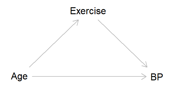
Now the interpretation above of a “one-year increase in age associated with a 0.5 increase in systolic blood pressure” isn’t quite correct, as instead this 0.5 increase is the direct effect of age on blood pressure not mediated by exercise. If we were interested in the total effect of age, given the DAG above this would simply be the association between age and blood pressure, without including exercise as a covariate in the model. The interpretation of the exercise coefficient is the total effect (and therefore is correct), as here age is a confounder of the exercise-blood pressure association, so would need to be adjusted for.
This highlights the importance of defining your estimand - the causal effect of interest - when the aim of the research is causal inference5. The choice of estimand will then inform the choice of statistical model one intends to run. For instance, in the simple example above, if our estimand is ‘the causal effect of age on blood pressure’ then, given our causal assumptions, there’s no need to adjust for exercise; but if our estimand is ‘the causal effect of exercise on blood pressure’, then we would need to adjust for age. You can’t include both age and exercise in the same model and interpret them both as total causal effects (which is the traditional ‘causal salad’ approach, where numerous variables are thrown into a regression model and interpreted without thinking about the causal structure of the data).
The table 2 fallacy is really rather pervasive, and is something I committed in my pre-causal days. For instance, in a paper looking at age at menarche, I explored whether previously reported effects of father absence accelerating age at menarche may in fact be due to differences in sibling relatedness and reproductive conflict6. Finding that father absence was not associated with age at menarche when including sibling relatedness as a covariate (which was associated with age at menarche), I concluded that sibling relatedness, rather than father absence, was associated with age at menarche.
However, thinking about the causal relations between these variables, it’s plausible that father absence may cause sibling relatedness. That is, father absence causes the mother to have a new relationship with someone else, meaning that future siblings will be half-siblings, rather than full siblings (of step-siblings, if the new partner already has children). This can be represented in a DAG like so:

In other words, in the paper I was treating sibling relatedness as a potential confounder, rather than a potential mediator, of the relationship between father absence and age at menarche. So by adjusting for sibling relatedness - assuming the hypothesised DAG is correct - I was in fact estimating the direct effect of father absence on age at menarche. The interpretation of the sibling relatedness coefficient can be interpreted as a total effect, but I should not have interpreted both father absence and sibling relatedness estimates as total effects. If I had thought about the causal structure of the data properly and clearly defined my estimand, this kind of misinterpretation could have been avoided7.
UK Race Report: Conflating confounders and mediators
Returning to the UK Government’s race report example, as Dagatha noted, the authors of the report seemingly treated socioeconomic background (SEB) as a confounder of the relationship between racial discrimination and inequality. As always, a DAG should make this clearer.
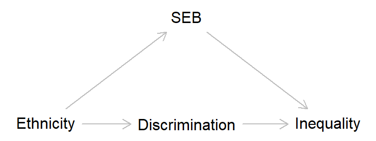
In this DAG, ‘Ethnicity’ is used as a proxy for ‘Discrimination’, so we have to estimate the direct effect of ethnicity on inequality in order to estimate the total effect of discrimination on inequality8. This DAG also shows that SEB confounds the association between ‘Discrimination’ and ‘Inequality’ - that is, there is an open back-door path from discrimination to inequality via ethnicity and SEB - so to establish the causal effect of ‘Discrimination’ on ‘Inequality’, we need to adjust for SEB. This is what the authors of the Race Report did, and found that most of association between race/ethnicity and inequality was explained by socioeconomic background (and other factors), rather than being due to discrimination.
However, if discrimination causes socioeconomic differences, then the picture changes considerably. Now, SEB is a mediator of how discrimination can lead to inequality, rather than a confounder. As we discussed above, to estimate the total effect of an exposure on an outcome in the presence of a mediator, we would not include the mediator in said model; if we did include it, we would instead only obtain the direct effect of discrimination on inequality (and if the effect of discrimination is fully mediated by SEB, this direct effect would be zero, just like we saw above in the example of blood pressure tablets and risk of heart attack).

Is there any evidence to suggest that SEB is a mediator rather than a confounder of the relationship between discrimination and inequality? In short, yes. For instance, residential segregation is a cause of ethnic differences in socioeconomic background. By treating SEB (and other factors) as confounders, rather than mediators, the Race Report was almost destined to underplay the seriousness of racial/ethnic discrimination on inequality9.
Summary
This post has covered:
- How to define ‘mediation’, which can only be defined in causal terms
- Identifying mediators in DAGs
- How adjusting for mediators can lead to biased total effect estimates
- The table 2 fallacy, and how ignoring the causal structure of the data and treating all regression coefficients as total effects can lead to incorrect conclusions
- The importance of clearly defining your estimand
- How confusing confounders and mediators can dramatically impact the interpretation of results
In the next post we’ll enter the murky world of colliders, explore how correlation can occur in the absence of causation, and examine how selection bias can bias our lovely inferences.
Further reading
Chapter 9 of Judea Pearl and Dana Mackenzie’s Book of Why is a good introduction to mediation (although it does get quite technical, especially when discussing causal mediation analysis).
Tyler VanderWeele’s book Explanation in Causal Inference: Methods for Mediation and Interaction is the bible on causal mediation analysis.
David Kenny’s webpage on mediation is also a nice introduction to all things mediation.
Daniel Westreich and Sander Greenland’s paper on the Table 2 fallacy should be essential reading too.
Stata code
*** Blood pressure tablets and heart attack example

* Clear data, set observations and set seed
clear
set obs 10000
set seed 5678

* Simulate taking BP tablets (caused by nothing/random
* assignment)
gen tablets = rbinomial(1, 0.5)
tab tablets

* Simulate post-tablet systolic blood pressure (lower in
* those taking tablets)
gen bp = 160 + (-20 * tablets) + rnormal(0, 10)
sum bp

* And now simulate having had a heart attack (only
* caused by blood pressure)
gen attack_p = invlogit(log(0.0001) + (log(1.05) * bp))
gen attack = rbinomial(1, attack_p)
tab attack

* Logistic regression of tablets on heart attack
* (estimating total effect of tablets on heart attack)
logistic attack tablets

* Logistic regression of tablets on heart attack
* including the mediator blood pressure (now estimating
* direct effect of tablets on heart attack)
logistic attack tablets bp
I say ‘ordinarily’, as sometimes the direct effect, rather than the total effect, may be the estimate of interest.↩︎
Strictly speaking this isn’t quite correct, as this simple mediation formula only applies to linear models. But for the sake of the pedagogical point I’m making here, I hope you’ll forgive this minor transgression.↩︎
Echoing the footnote above, this standard mediation formula only applies to linear models in the absence of interactions, but it’s a useful starting point. Causal mediation analysis can include binary mediators and outcomes, but I’m not going to discuss them here (see the ‘Further reading’).↩︎
Often presented in table 2 of papers, hence the name of the fallacy.↩︎
I often get confused between ‘estimand’ (the causal effect of interest), ‘estimate’ (the parameter values of said estimand from the data), and ‘estimator’ (the method to obtain the estimate; e.g., linear regression). For a helpful memory aid, see this tweet↩︎
You don’t need to worry about the evolutionary logic behind these hypotheses. Feel free to replace the variable names with ‘X’, ‘Y’ and ‘Z’ if it helps.↩︎
Given this, there is likely to be a causal association between father absence and earlier at age menarche - at least in this sample, and assuming no other sources of bias - it’s just that much of this effect may be mediated by sibling relatedness.↩︎
This sounds a bit odd, but I hope it makes sense. For more info on calculating ‘discrimination effects’ using this approach, see page 3 of this paper↩︎
As always, the truth is likely to be more complicated. Socioeconomic background and other factors (geography, family, culture, religion, etc.) may be both confounders and mediators, making causal estimation even more difficult. But the aim of this post isn’t to definitely answer this thorny question - which I am far from qualified to do! - but rather to gently introduce the concept of ‘mediators’.↩︎